Lecture 1: Functions and Derivatives

Note: The lecture notes here are from Session 2022/2023.

Download the original PDF →

---

1.1 Functions and Derivatives

1.1.1 Limit of a Function

Why should we learn limits?

• Limits are needed to define differential calculus. Every application of differential equation assumes that the limits defining the terms in the equations exist.
• Limits are needed in integral calculus because an integral is defined over a range of variables, and this form the limits in the integrations.
• Limits are needed in many real-life calculations, e.g. calculation of continuously compounded interest, margin of error, half-life of drugs, or in any calculation where the rate of change is important. This is because the rate of change is the derivative of a representative function, and the derivative (differentiation) are built on the foundation concept of a limit.

What is limit in calculus?

• In mathematics, a limit is the value that a function or sequence "approaches" as the input or index approaches some value. Limits are essential to calculus and mathematical analysis, and are used to define continuity, derivatives, and integrals.

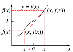
Suppose that the function $f(x)$ is defined for all values of $x$ near $a$, but not necessarily at $a$. As $x$ approaches $a$ (without attaining the value $a$), $f(x)$ approaches the number $L$. Then we can say that $L$ is the limit of $f(x)$ as $x$ approaches $a$, and write

$$\lim_{x \to a} f(x) = L$$

Figure 1

A function $f$ has limit $L$ as $x$ approaches $a$ if and only if $f(x)$ has both a left and a right limit as $x$ approaches $a$ and these one-sided limits both equal $L$. That is:

$$\lim_{x \to a} f(x) = L \iff \lim_{x \to a^+} f(x) = \lim_{x \to a^-} f(x) = L$$

• Note that, using the formal definition, there is no need to evaluate $f(a)$; indeed, $f(a)$ may or may not equal $L$. The limiting value of $f$ as $x \to a$ depends only on nearby values!

1.1.2 Limit Laws

We now look at the limit laws which define the individual properties of limits. Suppose that $C$ is a constant and the limits $\lim_{x \to a} f(x)$ and $\lim_{x \to a} g(x)$ exist. Then

Limit Law	Limit Law in symbols
Sum law	$\displaystyle \lim_{x \to a}[f(x) + g(x)] = \lim_{x \to a} f(x) + \lim_{x \to a} g(x)$
Difference law	$\displaystyle \lim_{x \to a}[f(x) - g(x)] = \lim_{x \to a} f(x) - \lim_{x \to a} g(x)$
Constant multiple law	$\displaystyle \lim_{x \to a} cf(x) = c\lim_{x \to a} f(x)$
Product law	$\displaystyle \lim_{x \to a}[f(x)g(x)] = \lim_{x \to a} f(x) \cdot \lim_{x \to a} g(x)$
Quotient law	$\displaystyle \lim_{x \to a}\frac{f(x)}{g(x)} = \frac{\lim_{x \to a} f(x)}{\lim_{x \to a} g(x)} \quad \text{if } \lim_{x \to a} g(x) \neq 0$
Power law	$\displaystyle \lim_{x \to a}[f(x)]^n = \left[\lim_{x \to a} f(x)\right]^n$

Questions:

1. What is limit of a constant function?

   Solution

   $\lim_{x \to a} c = c$

2. What is the limit of a linear function?

   Solution

   $\lim_{x \to a} x = a$

1.1.3 Evaluate Limit of a Function

If the function (be it linear, polynomial or rational function) is continuous at $x = a$, we can use "direct substitution" to evaluate a limit.

Example 1.1.1

Evaluate $\displaystyle \lim_{x \to 3}(2x+5)$.

Solution

$\lim_{x \to 3}(2x+5) = \lim_{x \to 3}(2x) + \lim_{x \to 3}(5) = 2\lim_{x \to 3}(x) + \lim_{x \to 3}(5) = 2(3) + 5 = 11$

Example 1.1.2

Evaluate $\displaystyle \lim_{x \to 3}(5x^2)$.

Solution

$\lim_{x \to 3}(5x^2) = 5\lim_{x \to 3}(x^2) = 5(3)^2 = 45$

Example 1.1.3

Evaluate $\displaystyle \lim_{x \to -2}\frac{x^2+8x-20}{x-2}$.

Solution

$$\begin{aligned} \lim_{x \to -2}\frac{x^2+8x-20}{x-2} &= \frac{(-2)^2 + 8(-2) - 20}{(-2) - 2} \\ &= \frac{4-16-20}{-4} = \frac{-32}{-4} = 8 \end{aligned}$$

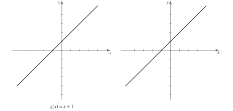
As we have seen, we may easily evaluate the limits of polynomials and limits of some (but not all) rational functions by direct substitution. However, it is certainly possible for $\lim_{x \to a} f(x)$ to exist when $f(a)$ is undefined, i.e. $f$ is discontinuous at $a$. For example:

Figure 2

If for all $x \neq a$, $f(x) = g(x)$ over some open interval containing $a$, then $\lim_{x \to a} f(x) = \lim_{x \to a} g(x)$. Usually, we can evaluate the limit by factoring or by rationalizing.

Example 1.1.4: Evaluate by factoring

Evaluate $\displaystyle \lim_{x \to 1}\frac{x^2-1}{x-1}$.

Solution

$\lim_{x \to 1}\frac{x^2-1}{x-1} = \lim_{x \to 1}\frac{(x-1)(x+1)}{x-1} = \lim_{x \to 1}(x+1) = 1+1 = 2$

Example 1.1.5: Evaluate by rationalizing

Evaluate $\displaystyle \lim_{t \to 0}\frac{\sqrt{t^2+9}-3}{t^2}$.

Solution

$$\begin{aligned} \lim_{t \to 0}\frac{\sqrt{t^2+9}-3}{t^2} &= \lim_{t \to 0}\frac{\sqrt{t^2+9}-3}{t^2} \times \frac{\sqrt{t^2+9}+3}{\sqrt{t^2+9}+3} \\ &= \lim_{t \to 0}\frac{(t^2+9)-9}{t^2\left(\sqrt{t^2+9}+3\right)} \\ &= \lim_{t \to 0}\frac{1}{\sqrt{t^2+9}+3} \\ &= \frac{1}{\sqrt{(0)^2+9}+3} = \frac{1}{6} \end{aligned}$$

Example 1.1.6

Find $\displaystyle \lim_{x \to 4}\frac{\sqrt{x}-2}{x-4}$.

Solution

$$\lim_{x \to 4}\frac{\sqrt{x}-2}{x-4} = \lim_{x \to 4}\frac{\sqrt{x}-2}{(\sqrt{x})^2-2^2} = \lim_{x \to 4}\frac{\sqrt{x}-2}{(\sqrt{x}+2)(\sqrt{x}-2)} = \lim_{x \to 4}\frac{1}{\sqrt{x}+2} = \frac{1}{\sqrt{4}+2} = \frac{1}{4}$$

Note: This problem can also be solved by rationalizing, please try on your own.

Example 1.1.7

Find $\displaystyle \lim_{x \to 2}\frac{\sqrt{x+7}-3}{\sqrt{x+2}-2}$.

Solution

$$\begin{aligned} \lim_{x \to 2}\frac{\sqrt{x+7}-3}{\sqrt{x+2}-2} &= \lim_{x \to 2}\frac{\sqrt{x+7}-3}{\sqrt{x+2}-2} \times \frac{\sqrt{x+2}+2}{\sqrt{x+2}+2} \times \frac{\sqrt{x+7}+3}{\sqrt{x+7}+3} \\ &= \lim_{x \to 2}\frac{(x-2)\left(\sqrt{x+2}+2\right)}{(x-2)\left(\sqrt{x+7}+3\right)} \\ &= \frac{\sqrt{2+2}+2}{\sqrt{2+7}+3} = \frac{4}{6} = \frac{2}{3} \end{aligned}$$

1.1.4 Limit for Trigonometric Function

We can replace a limit problem with another that may be simpler to solve. L'Hospital's Rule tells us that if we have an indeterminate form $0/0$ or $\infty/\infty$, all we need to do is differentiate the numerator and differentiate the denominator and then take the limit.

Suppose that we have one of the following cases,

$$\lim_{x \to a}\frac{f(x)}{g(x)} = \frac{0}{0} \quad \text{or} \quad \lim_{x \to a}\frac{f(x)}{g(x)} = \frac{\pm\infty}{\pm\infty}$$

where $a$ can be any real number, infinity or negative infinity. In these cases, we have

$$\lim_{x \to a}\frac{f(x)}{g(x)} = \lim_{x \to a}\frac{f'(x)}{g'(x)} \qquad \text{according to L'Hospital's Rule}$$

For example, evaluate $\displaystyle \lim_{\theta \to 0}\left(\frac{\sin\theta}{\theta}\right)$. We can see that this is a $0/0$ indeterminate form so let's just apply L'Hospital's Rule:

$$\lim_{\theta \to 0}\left(\frac{\sin\theta}{\theta}\right) = \lim_{\theta \to 0}\frac{(\sin\theta)'}{\theta'} = \lim_{\theta \to 0}\left(\frac{\cos\theta}{1}\right) = \frac{1}{1} = 1$$

$\displaystyle \lim_{\theta \to 0}\left(\frac{\sin\theta}{\theta}\right) = 1$ plays an important role in solving for other trigonometric limits.

$$\lim_{x \to 0}\cos x = 1 \qquad \text{and} \qquad \lim_{\theta \to 0}\left(\frac{\sin\theta}{\theta}\right) = 1 = \lim_{\theta \to 0}\left(\frac{\theta}{\sin\theta}\right)$$

Example 1.1.8

Find $\displaystyle \lim_{x \to 0}\left(\frac{\sin 3x}{4x}\right)$.

Solution

$$\begin{aligned} \lim_{x \to 0}\left(\frac{\sin 3x}{4x}\right) = \lim_{x \to 0}\frac{\left(\frac{\sin 3x}{3x}\right) \times 3x}{\left(\frac{\sin 4x}{4x}\right) \times 4x} = \lim_{x \to 0}\frac{3}{4} = \frac{3}{4} \end{aligned}$$

Alternatively, use L'Hospital's Rule:

$$\lim_{x \to 0}\left(\frac{\sin 3x}{4x}\right) = \lim_{x \to 0}\frac{(\sin 3x)'}{(4x)'} = \lim_{x \to 0}\frac{3\cos 3x}{4} = \frac{3\cos(0)}{4} = \frac{3}{4}$$

Example 1.1.9

Find $\displaystyle \lim_{x \to 0} x\cot(2x)$.

Solution

$$\begin{aligned} \lim_{x \to 0} x\cot(2x) &= \lim_{x \to 0}\frac{x\cos 2x}{\sin 2x} \\ &= \lim_{x \to 0}\frac{x\cos 2x}{\sin 2x} \times \frac{2}{2} \\ &= \lim_{x \to 0}\frac{1}{2}\cos 2x = \frac{1}{2}\cos 0 = \frac{1}{2} \end{aligned}$$

1.1.5 Continuity of Functions

Below shows several continuous functions (Figure 3). These functions are said to be continuous since their graphs have no "breaks", "gaps" or "holes".

Figure 3: Continuous functions

The graph of discontinuous function has breaks, gaps or points at which the function is undefined. For example, the function below (Figure 4) is undefined at $x=2$, i.e. the graph has a hole at $x=2$ and therefore is said to be discontinuous.

Figure 4: Discontinuous function with a gap at x=2.

A discontinuous function may also have different left- and right-hand limits as shown by Figure 5, therefore the limit at $x=3$ does not exist.

Figure 5: A discontinuous function with different left- and right-hand limits.

In other cases (Figure 6), the limits of the function at $x=2$ exist but is not equal to the value of the function at $x=2$. This function is also discontinuous.

Figure 6: A discontinuous function where the limit at x=2 exists but is not equal to the value of the function at x=2.

Figure 7 shows a function whereby the limits of the function at $x=3$ does not exist since the function either increases or decreases indefinitely at both sides of $x=3$. This is also a discontinuous function.

Figure 7: The limit at x=3 does not exist, as the function increases or decreases indefinitely on either side of x=3.

Taking into consideration all the information gathered from the examples of continuous and discontinuous functions shown above, we define a continuous function as follows.

Function $f$ is continuous at a point $a$ if the following conditions are satisfied:

1. $f(a)$ is defined
2. $\displaystyle \lim_{x \to a} f(x)$ exists
3. $\displaystyle \lim_{x \to a} f(x) = f(a)$

1.1.6 Derivatives: Basic Ideas and Definitions

The computation of the slope of a tangent line, the instantaneous rate of change of a function, and the instantaneous velocity of an object at $x = a$ all required us to compute the following limit:

$$\lim_{x \to a}\frac{f(x)-f(a)}{x-a} \qquad (1)$$

We also saw that with a small change of notation this limit could also be written as,

$$\lim_{h \to 0}\frac{f(a+h)-f(a)}{h} \qquad (2)$$

This is such an important limit, and it arises in so many places that we give it a name. We call it a derivative, which tells us the slope or rate of change of a function at any point. Here is the official definition of the derivative:

The derivative of $f(x)$ with respect to $x$ is the function $f'(x)$ and is defined as,

$$f'(x) = \lim_{h \to 0}\frac{f(x+h)-f(x)}{h} \qquad (3)$$

Note that we replaced all the $a$'s in (1) with $x$'s to acknowledge the fact that the derivative is really a function as well. We often "read" $f'(x)$ as "f prime of x".

Example 1.1.10

Find the derivative of the following function using the definition of the derivative.

$f(x) = 2x^2 - 16x + 35$

Solution

All we really need to do is to plug this function into the definition of the derivative, (3), and do some algebra.

$$\begin{aligned} f'(x) &= \lim_{h \to 0}\frac{f(x+h)-f(x)}{h} \\ &= \lim_{h \to 0}\frac{2(x+h)^2 - 16(x+h) + 35 - (2x^2 - 16x + 35)}{h} \\ &= \lim_{h \to 0}\frac{2x^2 + 4xh + 2h^2 - 16x - 16h + 35 - 2x^2 + 16x - 35}{h} \\ &= \lim_{h \to 0}\frac{h(4x + 2h - 16)}{h} \\ &= \lim_{h \to 0}(4x + 2h - 16) \\ &= 4x - 16 \end{aligned}$$

1.1.7 Rules of Differentiations

Here are useful rules to help you work out the derivatives of many functions. Note: the little mark $'$ means derivative of, and $f$ and $g$ are functions.

Common Functions	Function	Derivative
Constant	$c$	$0$
Line	$x$	$1$
Line	$ax$	$a$
Square	$x^2$	$2x$
Square Root	$\sqrt{x}$	$\left(\tfrac{1}{2}\right)x^{-1/2}$
Exponential	$e^x$	$e^x$
Exponential	$a^x$	$\ln(a)\,a^x$
Logarithms	$\ln(x)$	$1/x$
Logarithms	$\log_a(x)$	$1/(x\ln(a))$
Trigonometry ($x$ is in radians)	$\sin(x)$	$\cos(x)$
Trigonometry ($x$ is in radians)	$\cos(x)$	$-\sin(x)$
Trigonometry ($x$ is in radians)	$\tan(x)$	$\sec^2(x)$
Inverse Trigonometry	$\sin^{-1}(x)$	$1/\sqrt{1-x^2}$
Inverse Trigonometry	$\cos^{-1}(x)$	$-1/\sqrt{1-x^2}$
Inverse Trigonometry	$\tan^{-1}(x)$	$1/(1+x^2)$

Rules	Function	Derivative
Multiplication by constant	$cf$	$cf'$
Power Rule	$x^n$	$nx^{n-1}$
Sum Rule	$f+g$	$f' + g'$
Difference Rule	$f-g$	$f' - g'$
Product Rule	$fg$	$fg' + f'g$
Quotient Rule	$f/g$	$\dfrac{f'g - g'f}{g^2}$
Reciprocal Rule	$1/f$	$-f'/f^2$

"The derivative of" is also written $\dfrac{d}{dx}$.

So $\dfrac{d}{dx}\sin(x)$ and $\sin(x)'$ both mean "The derivative of $\sin(x)$".

1.1.8 Chain Rule

A function is composite if you can write it as $f(g(x))$. In other words, it is a function within a function.

For example, $\cos(x^2)$ is composite, because if we let $f(x) = \cos(x)$ and $g(x) = x^2$, then $\cos(x^2) = f(g(x))$. $g$ is the function within $f$, so we call $g$ the "inner" function and $f$ the "outer" function.

In calculus, the chain rule is a formula that expresses the derivative of a composite function (consisting of two differentiable functions $f$ and $g$) in terms of the derivatives of $f$ and $g$. In other words, we use chain rule to differentiate a composite function. The chain rule states that if $h(x) = f(g(x))$,

$$h'(x) = f'(g(x)) \cdot g'(x) \qquad \text{(Lagrange's notation)}$$

Or

$$\frac{dh}{dx} = \frac{df}{dg} \cdot \frac{dg}{dx} \qquad \text{(Leibniz's notation)}$$

Let's see how the chain rule is applied by differentiating $h(x) = (5-6x)^5$. Notice that $h$ is a composite function:

$h(x) = \overbrace{\left(\underbrace{5-6x}_{\text{inner}}\right)^{5}}^{\text{outer}}$

which can be expressed as $g(x) = u = 5-6x$ to represent the inner function and $f(u) = u^5$ to represent the outer function. Because $h$ is a composite function, we can differentiate it using the chain rule. Before applying the rule, let's find the derivatives of the inner and outer functions:

$g'(x) = -6 \qquad f'(u) = 5u^4$

Now let's apply chain rule:

$$\begin{aligned} h'(x) &= f'(u) \cdot g'(x) \\ &= 5(5-6x)^4 \cdot (-6) \\ &= -30(5-6x)^4 \end{aligned}$$

Example 1.1.11

Find $F'(x)$ if $F(x) = \sqrt{x^2+1}$.

Solution

We can express $F$ as

$F(x) = \sqrt{x^2+1} = f(g(x)) \quad \text{where} \quad f(u) = \sqrt{u} \ \text{ and } \ g(x) = u = x^2+1$

Since

$f'(u) = \frac{1}{2}u^{-1/2} = \frac{1}{2\sqrt{u}} \quad \text{and} \quad g'(x) = 2x$

Therefore,

$F'(x) = f'(g(x)) \cdot g'(x) = \frac{1}{2\sqrt{u}} \cdot 2x = \frac{x}{\sqrt{x^2+1}}$

Example 1.1.12

Find $f'(x)$ if $\displaystyle f(x) = \frac{1}{\sqrt[3]{x^2+x+1}}$.

Solution

$$\begin{aligned} f(x) &= (x^2+x+1)^{-1/3} \\ f'(x) &= -\frac{1}{3}(x^2+x+1)^{-4/3}\,\frac{d}{dx}(x^2+x+1) \\ &= -\frac{1}{3}(x^2+x+1)^{-4/3}(2x+1) \\ &= \frac{-2x-1}{3}(x^2+x+1)^{-4/3} \end{aligned}$$

Example 1.1.13

Find the derivative of a function $\displaystyle g(t) = \left(\frac{t-2}{2t+1}\right)^9$.

Solution

$$\begin{aligned} g'(t) &= 9\left(\frac{t-2}{2t+1}\right)^8 \frac{d}{dt}\left(\frac{t-2}{2t+1}\right) \\ &= 9\left(\frac{t-2}{2t+1}\right)^8 \frac{(1)(2t+1) - (t-2)(2)}{(2t+1)^2} \\ &= 9\left(\frac{t-2}{2t+1}\right)^8 \frac{5}{(2t+1)^2} \\ &= \frac{45(t-2)^8}{(2t+1)^{10}} \end{aligned}$$

1.1.9 Higher Derivatives

We take derivatives of functions. Since the derivative of a function is itself a function, we can take the derivative again. A higher-order derivative refers to the repeated process of taking derivatives of derivatives. Higher-order derivatives are applied to sketch curves, motion problems, and other applications.

Notation for higher-order derivatives:

	First Derivative	Second Derivative	Third Derivative	Fourth Derivative	Fifth Derivative
Leibniz (expanded)	$\dfrac{dy}{dx}$	$\dfrac{d}{dx}\left(\dfrac{dy}{dx}\right)$	$\dfrac{d}{dx}\left(\dfrac{d}{dx}\left(\dfrac{dy}{dx}\right)\right)$	$\dfrac{d}{dx}\left(\dfrac{d}{dx}\left(\dfrac{d}{dx}\left(\dfrac{dy}{dx}\right)\right)\right)$	$\dfrac{d}{dx}\left(\dfrac{d}{dx}\left(\dfrac{d}{dx}\left(\dfrac{d}{dx}\left(\dfrac{dy}{dx}\right)\right)\right)\right)$
Leibniz	$\dfrac{dy}{dx}$	$\dfrac{d^2y}{dx^2}$	$\dfrac{d^3y}{dx^3}$	$\dfrac{d^4y}{dx^4}$	$\dfrac{d^5y}{dx^5}$
Prime	$f'(x)$	$f''(x)$	$f'''(x)$	$f^{(4)}(x)$	$f^{(5)}(x)$
Euler	$D_xy$	$D_x^2y$	$D_x^3y$	$D_x^4y$	$D_x^5y$
Newton	$y'$	$y''$	$y'''$	$y^{(4)}$	$y^{(5)}$

Example 1.1.14

Find the third derivative of $\displaystyle f(x) = \frac{2\pi^2}{6-x}$.

Solution

Instead of using the quotient rule, we can simplify the function to

$f(x) = 2\pi^2(6-x)^{-1}$

$$\begin{aligned} f'(x) &= -2\pi^2(6-x)^{-2}(-1) = 2\pi^2(6-x)^{-2} \\ f''(x) &= -4\pi^2(6-x)^{-3}(-1) = 4\pi^2(6-x)^{-3} \\ f'''(x) &= -12\pi^2(6-x)^{-4}(-1) = 12\pi^2(6-x)^{-4} \end{aligned}$$

Example 1.1.15

Find the first four derivatives of $R(t) = 3t^2 + 8t^{1/2} + e^t$.

Solution

$$\begin{aligned} R'(t) &= 6t + 4t^{-1/2} + e^t \\ R''(t) &= 6 - 2t^{-3/2} + e^t \\ R'''(t) &= 3t^{-5/2} + e^t \\ R^{(4)}(t) &= -\frac{15}{2}t^{-7/2} + e^t \end{aligned}$$

Example 1.1.16

Find $f'''(4)$ if $f(x) = \sqrt{x}$.

Solution

$$\begin{aligned} f(x) &= x^{1/2} \\ f'(x) &= \frac{1}{2}x^{-1/2} \\ f''(x) &= -\frac{1}{4}x^{-3/2} \\ f'''(x) &= \frac{3}{8}x^{-5/2} \end{aligned}$$

Hence,

$f'''(4) = \frac{3}{8}(4)^{-5/2} = \frac{3}{8}\left(\frac{1}{32}\right) = \frac{3}{256}$

1.1.10 Derivatives of Inverse Trigonometric and Hyperbolic Functions

The Inverse Trigonometric functions are also called arcus functions, cyclometric functions or anti-trigonometric functions. These functions are used to obtain angle for a given trigonometric value. Inverse trigonometric functions have various application in engineering, geometry, navigation etc.

Here are the derivatives of all six inverse trigonometric functions.

Function	Derivative
$\sin^{-1}x$	$\dfrac{1}{\sqrt{1-x^2}}$
$\cos^{-1}x$	$-\dfrac{1}{\sqrt{1-x^2}}$
$\tan^{-1}x$	$\dfrac{1}{1+x^2}$
$\csc^{-1}x$	$-\dfrac{1}{\lvert x\rvert\sqrt{x^2-1}}$
$\sec^{-1}x$	$\dfrac{1}{\lvert x\rvert\sqrt{x^2-1}}$
$\cot^{-1}x$	$-\dfrac{1}{1+x^2}$

Example 1.1.17

Differentiate the function $f(x) = \sin^{-1}(x^2-1)$.

Solution

$$f'(x) = \frac{1}{\sqrt{1-(x^2-1)^2}} \cdot \frac{d}{dx}(x^2-1) = \frac{1}{\sqrt{1-(x^4-2x^2+1)}} \cdot 2x = \frac{2x}{\sqrt{2x^2-x^4}}$$

Example 1.1.18

Calculate the derivative of $\displaystyle f(x) = \tan^{-1}\left(\frac{x^2}{2}\right)$.

Solution

$$f'(x) = \frac{1}{1+\left(\frac{x^2}{2}\right)^2} \cdot \frac{d}{dx}\left(\frac{x^2}{2}\right) = \frac{1}{1+\left(\frac{x^2}{2}\right)^2} \cdot \frac{2x}{2} = \frac{x}{1+\left(\frac{x^2}{2}\right)^2} = \frac{x}{1+\frac{x^4}{4}}$$

Example 1.1.19

Calculate the derivative of $f(x) = x\sin^{-1}(3x)$.

Solution

$\frac{d}{dx}\sin^{-1}(3x) = \frac{1}{\sqrt{1-(3x)^2}} \cdot \frac{d}{dx}(3x) = \frac{3}{\sqrt{1-9x^2}}$

Hence,

$f'(x) = \frac{d}{dx}\left[x\sin^{-1}(3x)\right] = x \cdot \frac{3}{\sqrt{1-9x^2}} + (1)\sin^{-1}(3x) = \frac{3x}{\sqrt{1-9x^2}} + \sin^{-1}(3x)$

The derivatives of the hyperbolic functions are as following:

Function	Derivative
$\sinh x$	$\cosh x$
$\cosh x$	$\sinh x$
$\tanh x$	$\operatorname{sech}^2 x$
$\operatorname{csch} x$	$-\operatorname{csch} x \coth x$
$\operatorname{sech} x$	$-\operatorname{sech} x \tanh x$
$\coth x$	$-\operatorname{csch}^2 x$

Example 1.1.20

Differentiate $\dfrac{d}{dx}\cosh(\sqrt{x})$.

Solution

Any of the differentiation rule for the hyperbolic function can be combined with the chain rule. For instance,

$\frac{d}{dx}\cosh(\sqrt{x}) = \sinh(\sqrt{x}) \cdot \frac{d}{dx}(\sqrt{x}) = \sinh(\sqrt{x}) \cdot \frac{1}{2}x^{-1/2} = \frac{\sinh(\sqrt{x})}{2\sqrt{x}}$

Example 1.1.21

If $y = e^{\cosh 3x}$, find $y'$.

Solution

$y' = e^{\cosh 3x}\frac{d}{dx}\cosh(3x) = e^{\cosh 3x} \cdot \sinh(3x) \cdot \frac{d}{dx}(3x) = e^{\cosh 3x} \cdot \sinh(3x) \cdot 3 = 3e^{\cosh 3x}\sinh(3x)$

Example 1.1.22

If $y = \sinh(\cosh x)$, find $y'$.

Solution

$y' = \cosh(\cosh x) \cdot \frac{d}{dx}(\cosh x) = \cosh(\cosh x) \cdot \sinh(x)$

The inverse hyperbolic functions are all differentiable because the hyperbolic functions are differentiable.

Function	Derivative
$\sinh^{-1}x$	$\dfrac{1}{\sqrt{x^2+1}}$
$\cosh^{-1}x$	$\dfrac{1}{\sqrt{x^2-1}}$
$\tanh^{-1}x$	$\dfrac{1}{1-x^2}$
$\operatorname{csch}^{-1}x$	$-\dfrac{1}{\lvert x\rvert\sqrt{x^2+1}}$
$\operatorname{sech}^{-1}x$	$-\dfrac{1}{x\sqrt{1-x^2}}$
$\coth^{-1}x$	$\dfrac{1}{1-x^2}$

Example 1.1.23

Find the derivative of $y = -8\coth^{-1}(21x^3)$.

Solution

$y' = -8\left[\frac{1}{1-(21x^3)^2}\right]\frac{d}{dx}(21x^3) = \frac{-8}{1-441x^6} \cdot 63x^2 = \frac{-504x^2}{1-441x^6}$

1.1.11 Implicit Differentiation

The functions that we have seen so far can be described by expressing one variable explicitly in terms of another variable, for example $y = x$ or $y = x\sin x$.

Some functions, however, are defined implicitly by a relation between $x$ and $y$ such as

$x^2 + y^2 = 25 \qquad \text{or} \qquad x^3 + y^3 = 6xy$

The function is not written as "$y =$" some expression. This type of function is called implicit function. To differentiate implicit functions, we differentiate each side of an equation with two variables (usually $x$ and $y$) by treating one of the variables as a function of the other. Such differentiation is basically just a special kind of chain rule.

Let's differentiate $x^2 + y^2 = 1$ for example. Here, we treat $y$ as an implicit function of $x$.

$$\begin{aligned} x^2 + y^2 &= 1 \\ \frac{d}{dx}(x^2 + y^2) &= \frac{d}{dx}(1) \\ \frac{d}{dx}(x^2) + \frac{d}{dx}(y^2) &= 0 \\ 2x + 2y \cdot \frac{dy}{dx} &= 0 \\ \frac{dy}{dx} &= -\frac{x}{y} \end{aligned}$$

Notice that the derivative of $y^2$ is $2y \cdot \dfrac{dy}{dx}$ and not simply $2y$. This is because we treat $y$ as a function of $x$.

Example 1.1.24

Find $y'$ if $x^3 + y^3 = 6xy$, then find the tangent line to the curve at the point $(3,3)$.

Solution

Find $y'$:

$$\begin{aligned} \frac{d}{dx}x^3 + \frac{d}{dx}y^3 &= \frac{d}{dx}6xy \\ 3x^2 + 3y^2y' &= 6x \cdot 1 \cdot y' + 6 \cdot y \\ x^2 + y^2y' &= 2xy' + 2y \\ y^2y' - 2xy' &= 2y - x^2 \\ (y^2 - 2x)y' &= 2y - x^2 \\ y' &= \frac{2y - x^2}{y^2 - 2x} \end{aligned}$$

Find the tangent line to the curve at the point $(3,3)$:

$$\begin{aligned} y' &= \frac{2y-x^2}{y^2-2x} = \frac{2(3)-(3)^2}{3^2-2(3)} = -\frac{3}{3} = -1 \quad \text{(slope)} \\ y &= mx + c \\ 3 &= -1(3) + c \\ c &= 6 \end{aligned}$$

Hence, the tangent line is $y = -x + 6$.

Example 1.1.25

Find $y'$ if $\sin(x+y) = y^2\cos x$.

Solution

$$\begin{aligned} \frac{d}{dx}\sin(x+y) &= \frac{d}{dx}\left(y^2\cos x\right) \\ \cos(x+y) \cdot \frac{d}{dx}(x+y) &= (2y \cdot y')\cos x + y^2\frac{d}{dx}\cos x \\ \cos(x+y)(1+y') &= 2yy'\cos x + y^2(-\sin x) \\ \cos(x+y) + \cos(x+y)y' &= 2yy'\cos x - y^2\sin x \\ \cos(x+y)y' - 2y \cdot y'\cos x &= -y^2\sin x - \cos(x+y) \\ \left(\cos(x+y) - 2y\cos x\right)y' &= -y^2\sin x - \cos(x+y) \\ y' &= \frac{-y^2\sin x - \cos(x+y)}{\cos(x+y) - 2y\cos x} \end{aligned}$$

Example 1.1.26

Find $y''$ if $x^4 + y^4 = 16$.

Solution

$$\begin{aligned} \frac{d}{dx}(x^4 + y^4) &= \frac{d}{dx}(16) \\ 4x^3 + 4y^3 \cdot y' &= 0 \\ y' &= \frac{-4x^3}{4y^3} = -\frac{x^3}{y^3} \\ y'' &= \frac{-3x^2y^3 + 3y^2x^3y'}{y^6} \\ y'' &= \frac{-3x^2(y^4 + x^4)}{y^7} \end{aligned}$$

Example 1.1.27

Use implicit differentiation to find an equation of the tangent line to the curve at point $(1,1)$.

$x^2 + xy + y^2 = 3$

Solution

Use implicit differentiation:

$$\begin{aligned} 2x + xy' + y + 2y \cdot y' &= 0 \\ y' &= \frac{-y-2x}{x+2y} \end{aligned}$$

Substitute $(1,1)$ into $y'$:

$y' = \frac{-1-2(1)}{1+2(1)} = -1$

Substitute into line equation:

$$\begin{aligned} y &= mx + c \\ 1 &= -1(1) + c \\ c &= 2 \end{aligned}$$

Hence, tangent line is $y = -x + 2$.

Example 1.1.28

If $xy + y^3 = 1$, find value of $y''$ at the point where $x = 0$.

Solution

$$\begin{aligned} xy' + y + 3y^2y' &= 0 \\ (x + 3y^2)y' &= -y \\ y' &= -\frac{y}{x + 3y^2} \\ y'' &= \frac{-y'(x+3y^2) - (1 + 6yy')(-y)}{(x+3y^2)^2} = \frac{-y'(x+3y^2) + y(1 + 6yy')}{(x+3y^2)^2} \end{aligned}$$

At $x = 0$: $xy + y^3 = 1 \implies (0)y + y^3 = 1 \implies y = 1$.

$$\begin{aligned} y' &= -\frac{y}{x+3y^2} \implies y' = -\frac{1}{0+3(1)^2} = -\frac{1}{3} \\ y'' &= \frac{-\left(-\frac{1}{3}\right)\left(0+3(1)^2\right) + 1\left(1 + 6(1)\left(-\frac{1}{3}\right)\right)}{\left(0+3(1)^2\right)^2} = 0 \end{aligned}$$

Example 1.1.29

Assume that $y$ is a function of $x$. Find $y' = dy/dx$ for $e^{xy} = e^{4x} - e^{5y}$.

Solution

$$\begin{aligned} D(e^{xy}) &= D(e^{4x} - e^{5y}) \\ D(e^{xy}) &= D(e^{4x}) - D(e^{5y}) \\ e^{xy}D(xy) &= e^{4x}D(4x) - e^{5y}D(5y) \\ e^{xy}(x \cdot y' + (1)y) &= e^{4x}(4) - e^{5y}(5y') \\ xe^{xy}y' + ye^{xy} &= 4e^{4x} - 5y'e^{5y} \\ xe^{xy}y' + 5y'e^{5y} &= 4e^{4x} - ye^{xy} \\ (xe^{xy} + 5e^{5y})y' &= 4e^{4x} - ye^{xy} \\ y' &= \frac{4e^{4x} - ye^{xy}}{xe^{xy} + 5e^{5y}} \end{aligned}$$

1.1.12 Parametric Differentiation

Some relationships between two quantities or variables are so complicated that we sometimes introduce a third quantity or variable in order to make things easier to handle. In mathematics this third quantity is called a parameter. Instead of one equation relating say, $x$ and $y$, we have two equations, one relating $x$ with the parameter, and one relating $y$ with the parameter.

For example, the $x$ and $y$ coordinates of points on a curve can be defined in terms of a third variable, $t$, the parameter as follows:

$x = \cos(t) \qquad \text{and} \qquad y = \sin(t) \qquad \text{for } 0 \leq t \leq 2\pi$

Note how both $x$ and $y$ are given in terms of the third variable $t$.

It is often necessary to find the rate of change of a function (i.e. the curve) defined parametrically; that is, we want to calculate $dy/dx$. Let's look at one example how this is achieved.

Suppose we wish to find $\dfrac{dy}{dx}$ when $x = \cos t$ and $y = \sin t$. We differentiate both $x$ and $y$ with respect to the parameter, $t$:

$\frac{dx}{dt} = -\sin t \qquad \frac{dy}{dt} = \cos t$

From the chain rule, we know that

$\frac{dy}{dt} = \frac{dy}{dx}\frac{dx}{dt}$

so that, by rearrangement

$$\frac{dy}{dx} = \frac{\dfrac{dy}{dt}}{\dfrac{dx}{dt}} \qquad \text{provided } \frac{dx}{dt} \text{ is not equal to } 0$$

So, in this case

$\frac{dy}{dx} = \frac{\dfrac{dy}{dt}}{\dfrac{dx}{dt}} = \frac{\cos t}{-\sin t} = -\cot t$

Key Point

Parametric differentiation: if $x = x(t)$ and $y = y(t)$, then

$\frac{dy}{dx} = \frac{\dfrac{dy}{dt}}{\dfrac{dx}{dt}} \qquad \text{provided } \frac{dx}{dt} \neq 0$

Example 1.1.30

Find $dy/dx$ when $x = t^3 - t$ and $y = 4 - t^2$.

Solution

$$\begin{aligned} x &= t^3 - t & y &= 4 - t^2 \\ \frac{dx}{dt} &= 3t^2 - 1 & \frac{dy}{dt} &= -2t \end{aligned}$$

From the chain rule we have

$\frac{dy}{dx} = \frac{\dfrac{dy}{dt}}{\dfrac{dx}{dt}} = \frac{-2t}{3t^2 - 1}$

Example 1.1.31

Find $\dfrac{d^2y}{dx^2}$ when $x = t^3 + 3t^2$ and $y = t^4 - 8t^2$.

Solution

$\frac{dx}{dt} = 3t^2 + 6t \qquad \frac{dy}{dt} = 4t^3 - 16t$

Using the chain rule

$\frac{dy}{dx} = \frac{\dfrac{dy}{dt}}{\dfrac{dx}{dt}} \qquad \text{provided } \frac{dx}{dt} \neq 0$

So that

$$\frac{dy}{dx} = \frac{4t^3 - 16t}{3t^2 + 6t} = \frac{4t(t^2-4)}{3t(t+2)} = \frac{4t(t+2)(t-2)}{3t(t+2)} = \frac{4(t-2)}{3}$$

We can apply the chain rule a second time in order to find the second derivative, $\dfrac{d^2y}{dx^2}$:

$\frac{d^2y}{dx^2} = \frac{d}{dx}\left(\frac{dy}{dx}\right) = \frac{\dfrac{d}{dt}\left(\dfrac{dy}{dx}\right)}{\dfrac{dx}{dt}} = \frac{\dfrac{4}{3}}{3t^2+6t} = \frac{4}{9t(t+2)}$

---

1.2 Engineering Applications of Functions and Derivatives

1.2.1 Approximating Functions

We call the linear function

$L(x) = f(a) + f'(a)(x-a) \qquad (4)$

the linear approximation, or tangent line approximation, of $f$ at $x = a$. This function $L$ is also known as the linearization of $f$ at $x = a$. To show how useful the linear approximation can be, we look at how to find the linear approximation for $f(x) = \sqrt{x}$ at $x = 9$.

Example 1.2.1: Linear Approximation

Find the linear approximation of $f(x) = \sqrt{x}$ at $x = 9$ and use the approximation to estimate $\sqrt{9.1}$.

Solution

Since we are looking for the linear approximation at $x = 9$, using Equation (4), we know the linear approximation is given by

$L(x) = f(9) + f'(9)(x-9)$

We need to find $f(9)$ and $f'(9)$:

$f(x) = \sqrt{x} \implies f(9) = \sqrt{9} = 3$

$f'(x) = \frac{1}{2\sqrt{x}} \implies f'(9) = \frac{1}{2\sqrt{9}} = \frac{1}{6}$

Therefore, the linear approximation is given by,

$L(x) = 3 + \frac{1}{6}(x-9)$

Using the linear approximation, we can estimate $\sqrt{9.1}$ by writing

$\sqrt{9.1} = f(9.1) \approx L(9.1) = 3 + \frac{1}{6}(9.1-9) \approx 3.0167$

Exercise 1.2.1

Find the linear approximation of $f(x) = \sqrt[3]{x}$ at $x = 8$. Use it to approximate $\sqrt[3]{8.1}$ to five decimal places.

Solution

$L(x) = 2 + \frac{1}{12}(x-8); \qquad 2.00833$

Differentials

We have seen that linear approximations can be used to estimate function values. They can also be used to estimate the amount a function value changes as a result of a small change in the input. To discuss this more formally, we define a related concept: differentials. Differentials provide us with a way of estimating the amount a function changes as a result of a small change in input values.

When we first looked at derivatives, we used the Leibniz notation $dy/dx$ to represent the derivative of $y$ with respect to $x$. Although we used the expressions $dy$ and $dx$ in this notation, they did not have meaning on their own. Here we see a meaning to the expressions $dy$ and $dx$. Suppose $y = f(x)$ is a differentiable function. Let $dx$ be an independent variable that can be assigned any nonzero real number, and define the dependent variable $dy$ by

$dy = f'(x)\,dx \qquad (5)$

It is important to notice that $dy$ is a function of both $x$ and $dx$. The expressions $dy$ and $dx$ are called differentials. We can divide both sides of Equation (5) by $dx$, which yields

$\frac{dy}{dx} = f'(x) \qquad (6)$

This is the familiar expression we have used to denote a derivative. Equation (6) is known as the differential form of Equation (5).

Example 1.2.2: Computing Differentials

For each of the following functions, find $dy$ and evaluate when $x = 3$ and $dx = 0.1$.

a. $y = x^2 + 2x$ b. $y = \cos x$

Solution

The key step is calculating the derivative. When we have that, we can obtain $dy$ directly.

a. Since $f(x) = x^2 + 2x$, we know $f'(x) = 2x + 2$, and therefore $dy = (2x+2)\,dx$ When $x = 3$ and $dx = 0.1$, $dy = (2 \cdot 3 + 2)(0.1) = 0.8$

b. Since $f(x) = \cos x$, $f'(x) = -\sin(x)$. This gives us $dy = -\sin x\,dx$ When $x = 3$ and $dx = 0.1$ $dy = -\sin(3)(0.1) = -0.1\sin(3)$

Example 1.2.3: Approximating Change with Differentials

Let $y = x^2 + 2x$. Compute $\Delta y$ and $dy$ at $x = 3$ if $dx = 0.1$.

Solution

The actual change in $y$ if $x$ changes from $x = 3$ to $x = 3.1$ is given by

$\Delta y = f(3.1) - f(3) = \left[(3.1)^2 + 2(3.1)\right] - \left[3^2 + 2(3)\right] = 0.81$

The approximate change in $y$ is given by $dy = f'(3)\,dx$. Since $f'(x) = 2x + 2$, we have

$dy = f'(3)\,dx = (2(3)+2)(0.1) = 0.8$

Exercise 1.2.2

For $y = x^2 + 2x$, find $\Delta y$ and $dy$ at $x = 3$ if $dx = 0.2$.

Solution

$dy = 1.6, \qquad \Delta y = 1.64$

Calculating the Amount of Error

Any type of measurement is prone to a certain amount of error. In many applications, certain quantities are calculated based on measurements. For example, the area of a circle is calculated by measuring the radius of the circle. An error in the measurement of the radius leads to an error in the computed value of the area. Here we examine this type of error and study how differentials can be used to estimate the error.

Consider a function $f$ with an input that is a measured quantity. Suppose the exact value of the measured quantity is $a$ but the measured value is $a + dx$. We say the measurement error is $dx$ (or $\Delta x$). As a result, an error occurs in the calculated quantity $f(x)$. This type of error is known as a propagated error and is given by

$\Delta y = f(a + dx) - f(a) \qquad (7)$

Since all measurements are prone to some degree of error, we do not know the exact value of a measured quantity, so we cannot calculate the propagated error exactly. However, given an estimate of the accuracy of a measurement, we can use differentials to approximate the propagated error $\Delta y$. Specifically, if $f$ is a differentiable function at $a$, the propagated error is

$\Delta y \approx dy = f'(a)\,dx \qquad (8)$

Unfortunately, we do not know the exact value $a$. However, we can use the measured value $a + dx$, and estimate

$\Delta y \approx dy = f'(a + dx)\,dx \qquad (9)$

Example 1.2.4: Volume of Cube

Suppose the side length of a cube is measured to be $5\text{ cm}$ with an accuracy of $0.1\text{ cm}$.

a. Use differentials to estimate the error in the computed volume of the cube. b. Compute the volume of the cube if the side length is (i) $4.9\text{ cm}$ and (ii) $5.1\text{ cm}$ to compare the estimated error with the actual potential error.

Solution

a. The measurement of the side length is accurate to within $\pm 0.1\text{ cm}$. Therefore

$-0.1 \leq dx \leq 0.1$

The volume of a cube is given by $V = x^3$, which leads to

$dV = 3x^2\,dx$

Using the measured side length of $5\text{ cm}$, we can estimate that

$-3(5)^2(0.1) \leq dV \leq 3(5)^2(0.1)$

Therefore,

$-7.5 \leq dV \leq 7.5$

b. If the side length is actually $4.9\text{ cm}$, then the volume of the cube is $V(4.9) = (4.9)^3 = 117.649\text{ cm}^3$

If the side length is actually $5.1\text{ cm}$, then the volume of the cube is $V(5.1) = (5.1)^3 = 132.651\text{ cm}^3$

Therefore the actual volume of the cube is between $117.649$ and $132.651$. Since the side length is measured to be $5\text{ cm}$, the computed volume is $V(5) = (5)^3 = 125$. Therefore, the error in the computed volume is

$117.649 - 125 \leq dV \leq 132.651 - 125$

That is,

$-7.351 \leq dV \leq 7.651$

We see the estimated error $dV$ is relatively close to the actual potential error in the computed volume.

1.2.2 The Gradient of a Straight Line

To see how the derivative of $f$ can tell us where a function is increasing or decreasing, look at figure below. Between $A$ and $B$ and between $C$ and $D$, the tangent lines have positive slope and so $f'(x) > 0$. Between $B$ and $C$ the tangent lines have negative slope and so $f'(x) < 0$. Thus, it appears that $f$ increases when $f'(x)$ is positive and decreases when $f'(x)$ is negative.

To prove that this is always the case, we use the Mean Value Theorem.

Increasing/Decreasing Test

(a) If $f'(x) > 0$ on an interval, then $f$ is increasing on that interval.

(b) If $f'(x) < 0$ on an interval, then $f$ is decreasing on that interval.

The First Derivative Test

Suppose that $c$ is a critical number of a continuous function $f$.

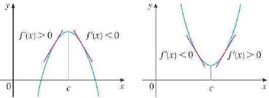
(a) If $f'$ changes from positive to negative at $c$, then $f$ has a local maximum at $c$.

(b) If $f'$ changes from negative to positive at $c$, then $f$ has a local minimum at $c$.

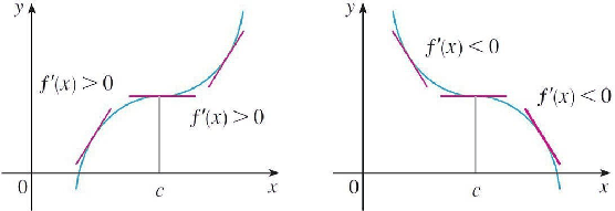
(c) If $f'$ does not change sign at $c$ (for example, if $f'$ is positive on both sides of $c$ or negative on both sides), then $f$ has no local maximum or minimum at $c$.

The First Derivative Test is a consequence of the Increase/Decrease Test. In part (a), for instance, since the sign of $f'(x)$ changes from positive to negative at $c$, $f$ is increasing to the left of $c$ and decreasing to the right of $c$. It follows that $f$ has a local maximum at $c$. It is easy to remember the First Derivative Test by visualizing diagrams such as those in figures below.

1.2.3 Concavity

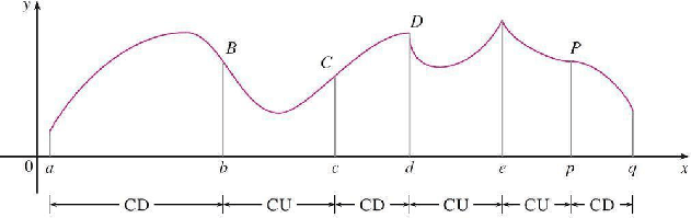
Figure below shows the graph of a function that is concave upward (CU) on intervals $(b,c)$, $(d,e)$, and $(e,p)$ and concave downward (CD) on intervals $(a,b)$, $(c,d)$ and $(p,q)$.

This reasoning can be reversed and suggests that the following theorem is true.

Concavity Test

(a) If $f''(x) > 0$ for all $x$ in $I$, then the graph of $f$ is concave upward on $I$.

(b) If $f''(x) < 0$ for all $x$ in $I$, then the graph of $f$ is concave downward on $I$.

The Second Derivative Test

Suppose $f''$ is continuous near $c$.

(a) If $f'(c) = 0$ and $f''(c) > 0$, then $f$ has a local minimum at $c$.

(b) If $f'(c) = 0$ and $f''(c) < 0$, then $f$ has a local maximum at $c$.

Example 1.2.5

Find local maximum and minimum values for function

$f(x) = 3x^4 - 4x^3 - 12x^2 + 5$

Solution

Find critical numbers:

$$\begin{aligned} f'(x) &= 12x^3 - 12x^2 - 24x \\ &= 12x(x^2 - x - 2) = 12x(x-2)(x+1) \end{aligned}$$

Critical numbers: $f'(x) = 0 \implies x = -1, 0, 2$

Perform the Increasing/Decreasing test on the critical numbers $(-1, 0, 2)$:

Interval	$12x$	$(x-2)$	$(x+1)$	$f'(x)$
$x < -1$	$-$	$-$	$-$	$f'(x) < 0$
$-1 < x < 0$	$-$	$-$	$+$	$f'(x) > 0$
$0 < x < 2$	$+$	$-$	$+$	$f'(x) < 0$
$x > 2$	$+$	$+$	$+$	$f'(x) > 0$

Hence,

• Local minimum at $x = -1$, $f(-1) = 0$
• Local maximum at $x = 0$, $f(0) = 5$
• Local minimum at $x = 2$, $f(2) = -27$

If we use the 2nd derivative test:

$f''(x) = 36x^2 - 24x - 24$

• $(x = -1) \implies f''(x)$ is $+$ve $\implies$ local minimum
• $(x = 0) \implies f''(x)$ is $-$ve $\implies$ local maximum
• $(x = 2) \implies f''(x)$ is $+$ve $\implies$ local minimum

Example 1.2.6

Discuss the curve $y = x^4 - 4x^3$ with respect to concavity, and local maxima and minima.

Solution

$$\begin{aligned} f(x) &= x^4 - 4x^3 \\ f'(x) &= 4x^3 - 12x^2 = 4x^2(x-3) \\ f''(x) &= 12x^2 - 24x = 12x(x-2) \end{aligned}$$

To find the critical numbers we set $f'(x) = 0$ and obtain $x = 0$ and $x = 3$.

To use the Second Derivative Test:

$f''(0) = 0 \qquad f''(3) = 36 > 0$

Since $f'(3) = 0$ and $f''(3) > 0$, $f(3) = -27$ is a local minimum. Since $f''(0) = 0$, the Second Derivative Test gives no information about the critical number $0$.

But since $f'(x) < 0$ for $x < 0$ and also for $0 < x < 3$, the First Derivative Test tells us that $f$ does not have a local maximum or minimum at $0$.

In fact, the expression for $f'(x)$ shows that $f$ decreases to the left of $3$ and increases to the right of $3$.

1.2.4 The Second Derivatives

Example 1.2.9

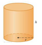
A manufacturer needs to make a cylindrical container that will hold 1.5 litres of liquid. Determine the dimensions (in cm) of the container that will minimize the amount of material used in its construction with a proof.

The next step is to create a corresponding mathematical model:

$\text{Minimize: } A = 2\pi r^2 + 2\pi rh \qquad \text{Constraint: } \pi r^2h = 1500$

i. Volume $= V = 1500$, find $h = ?$ ii. Find Area, $A(r)$ in terms of $r$ by substituting $h$. iii. Find $A'(r) = ?$ iv. Find critical numbers when $A'(r) = 0$. v. Prove critical number $\implies$ minimum point vi. Dimension $\implies$ radius and height

Solution

i. Volume, $V = \pi r^2h = 1500$

$h = \frac{1500}{\pi r^2}$

ii. Find Area $A(r)$ in terms of $r$ by substituting $h$.

$A(r) = 2\pi r^2 + 2\pi r\frac{1500}{\pi r^2} = 2\pi r^2 + \frac{3000}{r}$

iii. Find $A'(r) = ?$

$A'(r) = 4\pi r - 3000r^{-2} = \frac{4\pi r^3 - 3000}{r^2}$

iv. Find critical numbers when $A'(r) = 0$.

$\frac{4\pi r^3 - 3000}{r^2} = 0 \implies r = \sqrt[3]{\frac{3000}{4\pi}} = \sqrt[3]{238.7} \approx 6.20\text{ cm}$

v. Prove dimensions $\implies$ will give minimum value.

Using first derivative test: $A'(r) < 0$ for $r < \sqrt[3]{238.7}$ and $A'(r) > 0$ for $r > \sqrt[3]{238.7}$, so the critical number is a minimum point.

Or using second derivative test:

$A'(r) = 4\pi r - 3000r^{-2} \qquad A''(r) = 4\pi + 6000r^{-3} \to \text{positive} \implies \text{Min point}$

vi. Dimension:

$r \approx 6.20\text{ cm}, \qquad h = \frac{1500}{\pi r^2} \approx 12.41\text{ cm}$

Example 1.2.10

A window is being built. The bottom is a rectangle while the top is a semicircle. If there is $12\text{ m}$ of framing material, what must the dimensions of the window be in order to let in most light? Provide justification for resulted dimensions.

i. Find area and constraint. ii. Find Area, $A(r)$ in terms of $r$ by substituting $h$. iii. Find $A'(r) = ?$ iv. Find critical numbers when $A'(r) = 0$. v. Prove critical number $\implies$ max point vi. Dimension $\implies$ radius and height

Solution

i. Find area and constraint.

$A = 2rh + \frac{1}{2}\pi r^2$

$\text{Length} = 2h + 2r + \pi r = 12$

ii. Find Area, $A(r)$ in terms of $r$ by substituting $h$.

$h = \frac{12 - 2r - \pi r}{2} = 6 - r - \frac{\pi r}{2}$

$A(r) = 12r - r^2\left(2 + \frac{1}{2}\pi\right)$

iii. Find $A'(r) = ?$

$A'(r) = 12 - r(4 + \pi)$

iv. Find critical numbers when $A'(r) = 0$.

$12 - r(4+\pi) = 0 \implies r = \frac{12}{4+\pi}$

v. Prove critical number $\implies$ max point.

Use either first or second derivative test:

$A'(r) = 12 - r(4+\pi) \qquad A''(r) = -(4+\pi) \implies \text{negative} \implies \text{Max point}$

vi. Dimension of the window:

$\text{Width }(2r) = \frac{24}{4+\pi} \approx 3.36\text{ m}$

$\text{Height }(h) = 6 - r - \frac{\pi r}{2} \approx 1.68\text{ m}$

$\text{Curve} = \frac{12\pi}{4+\pi}$