Lecture 10: Multiple Integrals

Download the original PDF →

---

10.1 Double Integrals over Rectangles

10.1.1 Review of Definite Integrals

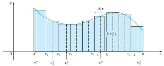
First let's recall the basic facts concerning definite integrals of functions of a single variable. If $f(x)$ is defined for $a \le x \le b$, we start by dividing the interval $[a, b]$ into $n$ subintervals $[x_{i-1}, x_i]$ of equal width $\Delta x = (b - a)/n$ and we choose sample points $x_i^*$ in these subintervals. Then we form the Riemann sum:

$\sum_{i=1}^{n} f(x_i^*)\Delta x \qquad \ldots (1)$

and take the limit of such sums as $n \to \infty$ to obtain the definite integral of $f$ from $a$ to $b$:

$\int_a^b f(x)\,dx = \lim_{n \to \infty}\sum_{i=1}^{n} f(x_i^*)\Delta x \qquad \ldots (2)$

In the special case where $f(x) \ge 0$, the Riemann sum can be interpreted as the sum of the areas of the approximating rectangles in Figure 10.1, and $\int_a^b f(x)\,dx$ represents the area under the curve $y = f(x)$ from $a$ to $b$.

Figure 10.1: Riemann sum approximation

10.1.2 Volumes and Double Integrals

In a similar manner we consider a function $f$ of two variables defined on a closed rectangle

$R = [a, b] \times [c, d] = \{(x, y) \in \mathbb{R}^2 \mid a \le x \le b,\ c \le y \le d\}$

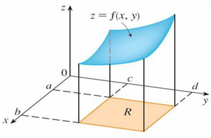
and we first suppose that $f(x, y) \ge 0$. The graph of $f$ is a surface with equation $z = f(x, y)$.

Let $S$ be the solid that lies above $R$ and under the graph of $f$, that is,

$S = \{(x, y, z) \in \mathbb{R}^3 \mid 0 \le z \le f(x, y),\ (x, y) \in R\} \qquad \text{(See Figure 10.2.)}$

Figure 10.2: f is a surface with equation z = f(x, y).

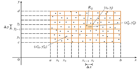
Our goal is to find the volume of $S$. The first step is to divide the rectangle $R$ into subrectangles. We accomplish this by dividing the interval $[a, b]$ into $m$ subintervals $[x_{i-1}, x_i]$ of equal width $\Delta x = (b - a)/m$ and dividing $[c, d]$ into $n$ subintervals $[y_{j-1}, y_j]$ of equal width $\Delta y = (d - c)/n$.

By drawing lines parallel to the coordinate axes through the endpoints of these subintervals, as in Figure 10.3, we form the subrectangles

$R_{ij} = [x_{i-1}, x_i] \times [y_{j-1}, y_j] = \{(x, y) \mid x_{i-1} \le x \le x_i,\quad y_{j-1} \le y \le y_j\}$

each with area $\Delta A = \Delta x \Delta y$.

Figure 10.3: Dividing R into subrectangles

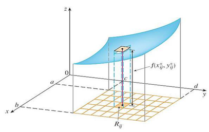
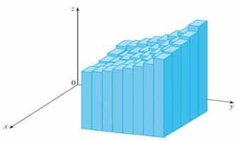
If we choose a sample point $(x_{ij}^*, y_{ij}^*)$ in each $R_{ij}$, then we can approximate the part of $S$ that lies above each $R_{ij}$ by a thin rectangular box (or "column") with base $R_{ij}$ and height $f(x_{ij}^*, y_{ij}^*)$ as shown in Figure 10.4.

The volume of this box is the height of the box times the area of the base rectangle:

$f(x_{ij}^*, y_{ij}^*)\Delta A$

Figure 10.4: Approximation by a thin rectangular box

If we follow this procedure for all the rectangles and add the volumes of the corresponding boxes, we get an approximation to the total volume of $S$:

$V \approx \sum_{i=1}^{m}\sum_{j=1}^{n} f(x_{ij}^*, y_{ij}^*)\,\Delta A \qquad (3)$

This double sum means that for each subrectangle we evaluate $f$ at the chosen point and multiply by the area of the subrectangle, and then we add the results. (See Figure 10.5.)

Figure 10.5: Approximation to the total volume of S

Our intuition tells us that the approximation given in Eq. (3) becomes better as $m$ and $n$ become larger and so we would expect that:

$V = \lim_{m, n \to \infty}\sum_{i=1}^{m}\sum_{j=1}^{n} f(x_{ij}^*, y_{ij}^*)\,\Delta A \qquad (4)$

We use the expression in Eq. (4) to define the volume (V) of the solid $S$ that lies under the graph of $f$ and above the rectangle $R$. Limits of the type that appear in Eq. (4) occur frequently, not just in finding volumes but in a variety of other situations even when $f$ is not a positive function. So we make the following definition.

Definition

The double integral of $f$ over the rectangle $R$ is

$\iint_R f(x, y)\,dA = \lim_{m, n \to \infty}\sum_{i=1}^{m}\sum_{j=1}^{n} f(x_{ij}^*, y_{ij}^*)\,\Delta A$

if this limit exists.

The precise meaning of the limit in Definition 5 is that for every number $\varepsilon > 0$ there is an integer $N$ such that

$\left| \iint_R f(x, y)\,dA - \sum_{i=1}^{m}\sum_{j=1}^{n} f(x_{ij}^*, y_{ij}^*)\,\Delta A \right| < \varepsilon$

for all integers $m$ and $n$ greater than $N$ and for any choice of sample points $(x_{ij}^*, y_{ij}^*)$ in $R_{ij}$. A function $f$ is called integrable if the limit in Definition 5 exists.

It is shown in courses on advanced calculus that all continuous functions are integrable. In fact, the double integral of $f$ exists provided that $f$ is "not too discontinuous." In particular, if $f$ is bounded on $R$, [that is, there is a constant $M$ such that $|f(x, y)| \le M$ for all $(x, y)$ in $R$], and $f$ is continuous there, except on a finite number of smooth curves, then $f$ is integrable over $R$.

The sample point $(x_{ij}^*, y_{ij}^*)$ can be chosen to be any point in the subrectangle $R_{ij}$, but if we choose it to be the upper right-hand corner of $R_{ij}$ [namely $(x_i, y_j)$, see Figure 10.3], then the expression for the double integral looks simpler:

$\iint_R f(x, y)\,dA = \lim_{m, n \to \infty}\sum_{i=1}^{m}\sum_{j=1}^{n} f(x_i, y_j)\,\Delta A \qquad (6)$

By comparing Eq. (4) and Definition 5, we see that a volume can be written as a double integral:

If $f(x, y) \ge 0$, then the volume $V$ of the solid that lies above the rectangle $R$ and below the surface $z = f(x, y)$ is

$V = \iint_R f(x, y)\,dA$

The sum in Definition 5,

$\sum_{i=1}^{m}\sum_{j=1}^{n} f(x_{ij}^*, y_{ij}^*)\,\Delta A$

is called a double Riemann sum and is used as an approximation to the value of the double integral. [Notice how similar it is to the Riemann sum in (1) for a function of a single variable.]. If $f$ happens to be a positive function, then the double Riemann sum represents the sum of volumes of columns, as in Figure 10.5, and is an approximation to the volume under the graph of $f$.

10.1.3 Iterated Integrals

Suppose that $f$ is a function of two variables that is integrable on the rectangle $R = [a, b] \times [c, d]$.

We use the notation $\int_c^d f(x, y)\,dy$ to mean that $x$ is held fixed and $f(x, y)$ is integrated with respect to $y$ from $y = c$ to $y = d$. This procedure is called partial integration with respect to y. (Notice its similarity to partial differentiation.)

Now $\int_c^d f(x, y)\,dy$ is a number that depends on the value of $x$, so it defines a function of $x$:

$A(x) = \int_c^d f(x, y)\,dy$

If we now integrate the function $A$ with respect to $x$ from $x = a$ to $x = b$, we get

$\int_a^b A(x)\,dx = \int_a^b\left[\int_c^d f(x, y)\,dy\right]dx \qquad (7)$

The integral on the right side of Eq. (7) is called an iterated integral. Usually the brackets are omitted. Thus

$\int_a^b\int_c^d f(x, y)\,dy\,dx = \int_a^b\left[\int_c^d f(x, y)\,dy\right]dx \qquad (8)$

means that we first integrate with respect to $y$ from $c$ to $d$ and then with respect to $x$ from $a$ to $b$.

Similarly, the iterated integral:

$\int_c^d\int_a^b f(x, y)\,dx\,dy = \int_c^d\left[\int_a^b f(x, y)\,dx\right]dy \qquad (9)$

means that we first integrate with respect to $x$ (holding $y$ fixed) from $x = a$ to $x = b$ and then we integrate the resulting function of $y$ with respect to $y$ from $y = c$ to $y = d$. Notice that in both Eq. (8) and (9) we work from the inside out.

The following theorem gives a practical method for evaluating a double integral by expressing it as an iterated integral (in either order).

Fubini's Theorem

If $f$ is continuous on the rectangle $R = \{(x, y) \mid a \le x \le b,\ c \le y \le d\}$, then

$\iint_R f(x, y)\,dA = \int_a^b\int_c^d f(x, y)\,dy\,dx = \int_c^d\int_a^b f(x, y)\,dx\,dy$

More generally, this is true if we assume that $f$ is bounded on $R$, $f$ is discontinuous only on a finite number of smooth curves, and the iterated integrals exist.

In the special case where $f(x, y)$ can be factored as the product of a function of $x$ only and a function of $y$ only, the double integral of $f$ can be written in a particularly simple form. To be specific, suppose that $f(x, y) = g(x)h(y)$ and $R = [a, b] \times [c, d]$. Then Fubini's Theorem gives

$\iint_R f(x, y)\,dA = \int_c^d\int_a^b g(x)h(y)\,dx\,dy = \int_c^d\left[\int_a^b g(x)h(y)\,dx\right]dy$

In the inner integral, $y$ is a constant, so $h(y)$ is a constant and we can write

$\int_c^d\left[\int_a^b g(x)h(y)\,dx\right]dy = \int_c^d\left[h(y)\left(\int_a^b g(x)\,dx\right)\right]dy = \int_a^b g(x)\,dx\int_c^d h(y)\,dy$

since $\int_a^b g(x)\,dx$ is a constant. Therefore, in this case, the double integral of $f$ can be written as the product of two single integrals:

$\iint_R g(x)h(y)\,dA = \int_a^b g(x)\,dx\int_c^d h(y)\,dy \qquad \text{where } R = [a, b] \times [c, d] \qquad (11)$

Example 10.1

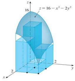
Find the volume of the solid that lies above the square $R = [0, 2] \times [0, 2]$ and below the elliptic paraboloid $z = 16 - x^2 - 2y^2$, as shown in Figure 10.6.

Figure 10.6: Volume of the approximating rectangular boxes

Solution

Solving using iterated integrals – Method 1

$$\begin{aligned} \text{Sum of volume} &= \int_0^2\int_0^2 16 - x^2 - 2y^2\,dx\,dy \\ &= \int_0^2\left[16x - \frac{x^3}{3} - 2xy^2\right]_0^2 dy \\ &= \int_0^2\left[\frac{88}{3} - 4y^2\right]_0^2 dy = \left[\frac{88}{3}y - \frac{4y^3}{3}\right]_0^2 = 48\ \text{unit}^3 \end{aligned}$$

Solving using iterated integrals – Method 2

$$\begin{aligned} \text{Sum of volume} &= \int_0^2\int_0^2 16 - x^2 - 2y^2\,dy\,dx \\ &= \int_0^2\left[16y - x^2y - \frac{2}{3}y^3\right]_0^2 dx \\ &= \int_0^2\left[\frac{80}{3} - 2x^2\right]_0^2 dx = \left[\frac{80}{3}x - \frac{2x^3}{3}\right]_0^2 = 48\ \text{unit}^3 \end{aligned}$$

Both method based on iterated integrals give the same answer.

Example 10.2

Evaluate the iterated integral:

$\int_0^3\int_1^2 x^2y\,dy\,dx$

Solution

Regarding $x$ as a constant, we obtain:

$$\begin{aligned} \int_1^2 x^2y\,dy &= \left[x^2\frac{y^2}{2}\right]_{y=1}^{y=2} \\ &= x^2\left(\frac{2^2}{2}\right) - x^2\left(\frac{1^2}{2}\right) = \frac{3}{2}x^2 \end{aligned}$$

Thus the function $A$ in the preceding discussion is given by $A(x) = \dfrac{3}{2}x^2$ in this example. We now integrate this function of $x$ from 0 to 3:

$$\begin{aligned} \int_0^3\int_1^2 x^2y\,dy\,dx &= \int_0^3\left[\int_1^2 x^2y\,dy\right]dx = \int_0^3 \frac{3}{2}x^2\,dx \\ &= \left.\frac{x^3}{2}\right|_0^3 = \frac{27}{2} \end{aligned}$$

10.1.4 Average Value

We know that the average value of a function $f$ of one variable defined on an interval $[a, b]$ is:

$f_{ave} = \frac{1}{b - a}\int_a^b f(x)\,dx$

Similarly, we define the average value of a function $f$ of two variables defined on a rectangle $R$ to be:

$f_{ave} = \frac{1}{A(R)}\iint_R f(x, y)\,dA$

where $A(R)$ is the area of $R$. If $f(x, y) \ge 0$, the equation:

$A(R) \times f_{ave} = \iint_R f(x, y)\,dA$

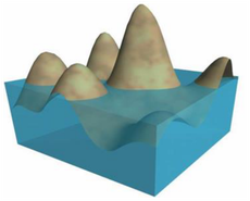
says that the box with base $R$ and height $f_{ave}$ has the same volume as the solid that lies under the graph of $f$. If $z = f(x, y)$ describes a mountainous region and you chop off the tops of the mountains at height $f_{ave}$, then you can use them to fill in the valleys so that the region becomes completely flat. See Figure 10.7.

Figure 10.7: Mountainous region

---

10.2 Double Integrals over General Regions

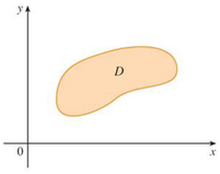
For single integrals, the region over which we integrate is always an interval. But for double integrals, we want to be able to integrate a function $f$ not just over rectangles but also over regions $D$ of more general shape, such as the one illustrated in Figure 10.8.

Figure 10.8: Regions D

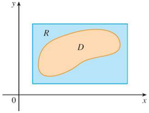
We suppose that $D$ is a bounded region, which means that $D$ can be enclosed in a rectangular region $R$ as in Figure 10.9.

Figure 10.9: Regions D enclosed in a rectangular region R

Then we define a new function $F$ with domain $R$ by:

$F(x, y) = \begin{cases} f(x, y) & \text{if } (x, y) \text{ is in } D \\ 0 & \text{if } (x, y) \text{ is in } R \text{ but not in } D \end{cases} \qquad \ldots (12)$

If $F$ is integrable over $R$, then we define the double integral of f over D by:

$\iint_D f(x, y)\,dA = \iint_R F(x, y)\,dA \qquad \ldots (13)$

Where $F$ is given by Eq. (12). Definition in Eq. (13) makes sense because $R$ is a rectangle and so $\iint_R F(x, y)\,dA$ has been previously defined. The procedure that we have used is reasonable because the values of $F(x, y)$ are 0 when $(x, y)$ lies outside $D$ and so they contribute nothing to the integral.

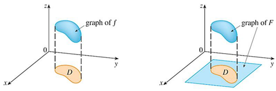
This means that it does not matter what rectangle $R$ we use as long as it contains $D$. In the case where $f(x, y) \ge 0$, we can still interpret $\iint_D f(x, y)\,dA$ as the volume of the solid that lies above $D$ and under the surface $z = f(x, y)$ (the graph of $f$).

You can see that this is reasonable by comparing the graphs of $f$ and $F$ in Figures 10.10 and remembering that $\iint_R F(x, y)\,dA$ is the volume under the graph of $F$.

Figure 10.10: Comparison between graphs of f and F

Figure 10.10 also shows that $F$ is likely to have discontinuities at the boundary points of $D$. Nonetheless, if $f$ is continuous on $D$ and the boundary curve of $D$ is "well behaved", then it can be shown that $\iint_R F(x, y)\,dA$ exists and therefore $\iint_D f(x, y)\,dA$ exists. In particular, this is the case for type I and type II regions.

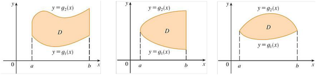
A plane region $D$ is said to be of type I if it lies between the graphs of two continuous functions of $x$, that is,

$D = \{(x, y) \mid a \le x \le b,\ g_1(x) \le y \le g_2(x)\}$

where $g_1$ and $g_2$ are continuous on $[a, b]$.

Some examples of type I regions are shown in Figure 10.11.

Figure 10.11: Examples of type I regions

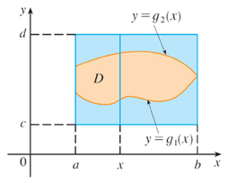
In order to evaluate $\iint_D f(x, y)\,dA$ when $D$ is a region of type I, we choose a rectangle $R = [a, b] \times [c, d]$ that contains $D$, as in Figure 10.12, and we let $F$ be the function given by Eq. (12); that is, $F$ agrees with $f$ on $D$ and $F$ is 0 outside $D$.

Figure 10.12: Examples of type I regions

Then, by Fubini's Theorem,

$\iint_D f(x, y)\,dA = \iint_R F(x, y)\,dA = \int_a^b\int_c^d F(x, y)\,dy\,dx$

Observe that $F(x, y) = 0$ if $y < g_1(x)$ or $y > g_2(x)$ because $(x, y)$ then lies outside $D$. Therefore,

$\int_c^d F(x, y)\,dy = \int_{g_1(x)}^{g_2(x)} F(x, y)\,dy = \int_{g_1(x)}^{g_2(x)} f(x, y)\,dy$

because $F(x, y) = f(x, y)$ when $g_1(x) \le y \le g_2(x)$. Thus we have the following formula that enables us to evaluate the double integral as an iterated integral.

If $f$ is continuous on a type I region $D$ such that

$D = \{(x, y) \mid a \le x \le b,\ g_1(x) \le y \le g_2(x)\}$

then

$\iint_D f(x, y)\,dA = \int_a^b\int_{g_1(x)}^{g_2(x)} f(x, y)\,dy\,dx \qquad \ldots (14)$

The integral on the right side of Eq. (14) is an iterated integral, except that in the inner integral we regard $x$ as being constant not only in $f(x, y)$ but also in the limits of integration, $g_1(x)$ and $g_2(x)$.

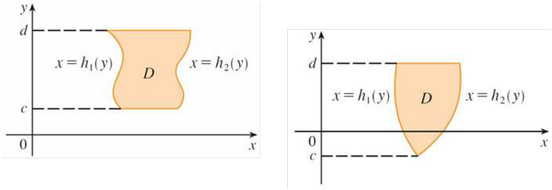
We also consider plane regions of type II, which can be expressed as:

$D = \{(x, y) \mid c \le y \le d,\ h_1(y) \le x \le h_2(y)\} \qquad \ldots (15)$

where $h_1$ and $h_2$ are continuous. Two such regions are illustrated in Figure 10.13.

Figure 10.13: Examples of type II regions

Using the same methods that were used in establishing Eq. (14), we can show that:

$\iint_D f(x, y)\,dA = \int_c^d\int_{h_1(y)}^{h_2(y)} f(x, y)\,dx\,dy \qquad \ldots (16)$

Where $D$ is a type II region given by Eq. (15).

Example 10.3

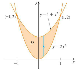
Evaluate $\iint_D (x + 2y)\,dA$, where $D$ is the region bounded by the parabolas $y = 2x^2$ and $y = 1 + x^2$.

Solution

The parabolas intersect when $2x^2 = 1 + x^2$, that is, $x^2 = 1$, so $x = \pm 1$.

We note that the region $D$, sketched in Figure 10.14, is a type I region but not a type II region and we can write:

$D = \{(x, y) \mid -1 \le x \le 1,\ 2x^2 \le y \le 1 + x^2\}$

Figure 10.14: Region D

Since the lower boundary is $y = 2x^2$ and the upper boundary is $y = 1 + x^2$, Eq. (14) gives:

$$\begin{aligned} \iint_D (x + 2y)\,dA &= \int_{-1}^1\int_{2x^2}^{1+x^2} (x + 2y)\,dy\,dx \\ &= \int_{-1}^1\left[xy + y^2\right]_{y=2x^2}^{y=1+x^2} dx \\ &= \int_{-1}^1\left[x(1 + x^2) + (1 + x^2)^2 - x(2x^2) - (2x^2)^2\right]dx \\ &= \int_{-1}^1(-3x^4 - x^3 + 2x^2 + x + 1)dx = \frac{32}{15} \end{aligned}$$

10.2.1 Properties of Double Integrals

We assume that all the following integrals exist. For rectangular regions $D$, the first three properties can be proved in the same manner. And then for general regions the properties follow from definition in Eq. (13).

$\iint_D \left[f(x, y) + g(x, y)\right]dA = \iint_D f(x, y)\,dA + \iint_D g(x, y)\,dA \qquad \ldots (17)$

$\iint_D cf(x, y)\,dA = c\iint_D f(x, y)\,dA \qquad \ldots (18)$

where $c$ is a constant. If $f(x, y) \ge g(x, y)$ for all $(x, y)$ in $D$, then:

$\iint_D f(x, y)\,dA \ge \iint_D g(x, y)\,dA \qquad \ldots (19)$

The next property of double integrals is similar to the property of single integrals given by the equation:

$\int_a^b f(x)\,dx = \int_a^c f(x)\,dx + \int_c^b f(x)\,dx.$

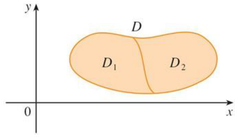
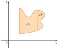
If $D = D_1 \cup D_2$, where $D_1$ and $D_2$ do not overlap except perhaps on their boundaries (see Figure 10.15), then

$\iint_D f(x, y)\,dA = \iint_{D_1} f(x, y)\,dA + \iint_{D_2} f(x, y)\,dA \qquad \ldots (20)$

Figure 10.15: Region D = D1 U D2

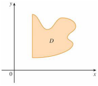
Property in Eq. (20) can be used to evaluate double integrals over regions $D$ that are neither type I nor type II but can be expressed as a union of regions of type I or type II. Figure 10.16 illustrates this procedure.

Figure 10.16

The next property of integrals says that if we integrate the constant function $f(x, y) = 1$ over a region $D$, we get the area of $D$:

$\iint_D 1\,dA = A(D)$

The last property states that:

If $m \le f(x, y) \le M$ for all $(x, y)$ in $D$, then

$mA(D) \le \iint_D f(x, y)\,dA \le MA(D)$

---

10.3 Triple Integrals

We have defined single integrals for functions of one variable and double integrals for functions of two variables, so we can define triple integrals for functions of three variables. Let's first deal with the simplest case where $f$ is defined on a rectangular box:

$B = \{(x, y, z) \mid a \le x \le b,\ c \le y \le d,\ r \le z \le s\} \qquad \ldots (21)$

The first step is to divide $B$ into sub-boxes. We do this by dividing the interval $[a, b]$ into $l$ subintervals $[x_{i-1}, x_i]$ of equal width $\Delta x$, dividing $[c, d]$ into $m$ subintervals of width $\Delta y$, and dividing $[r, s]$ into $n$ subintervals of width $\Delta z$.

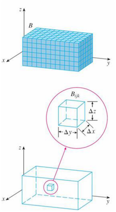
The planes through the endpoints of these subintervals parallel to the coordinate planes divide the box $B$ into $lmn$ sub-boxes

$B_{ijk} = [x_{i-1}, x_i] \times [y_{j-1}, y_j] \times [z_{k-1}, z_k]$

which are shown in Figure 10.24. Each sub-box has volume $\Delta V = \Delta x\,\Delta y\,\Delta z$.

Figure 10.24: Rectangular box

Then we form the triple Riemann sum:

$\sum_{i=1}^{l}\sum_{j=1}^{m}\sum_{k=1}^{n} f(x_{ijk}^*, y_{ijk}^*, z_{ijk}^*)\,\Delta V \qquad \ldots (22)$

where the sample point $(x_{ijk}^*, y_{ijk}^*, z_{ijk}^*)$ is in $B_{ijk}$. By analogy with the definition of a double integral, we define the triple integral as the limit of the triple Riemann sums in Eq. (22).

Definition

The triple integral of $f$ over the box $B$ is

$\iiint_B f(x, y, z)\,dV = \lim_{l, m, n \to \infty}\sum_{i=1}^{l}\sum_{j=1}^{m}\sum_{k=1}^{n} f(x_{ijk}^*, y_{ijk}^*, z_{ijk}^*)\,\Delta V$

if this limit exists.

Again, the triple integral always exists if $f$ is continuous. We can choose the sample point to be any point in the sub-box, but if we choose it to be the point $(x_i, y_j, z_k)$ we get a simpler-looking expression:

$\iiint_B f(x, y, z)\,dV = \lim_{l, m, n \to \infty}\sum_{i=1}^{l}\sum_{j=1}^{m}\sum_{k=1}^{n} f(x_i, y_j, z_k)\,\Delta V$

Just as for double integrals, the practical method for evaluating triple integrals is to express them as iterated integrals as follows:

Fubini's Theorem for Triple Integrals

If $f$ is continuous on the rectangular box $B = [a, b] \times [c, d] \times [r, s]$, then

$\iiint_B f(x, y, z)\,dV = \int_r^s\int_c^d\int_a^b f(x, y, z)\,dx\,dy\,dz$

The iterated integral on the right side of Fubini's Theorem means that we integrate first with respect to $x$ (keeping $y$ and $z$ fixed), then we integrate with respect to $y$ (keeping $z$ fixed), and finally we integrate with respect to $z$. There are five other possible orders in which we can integrate, all of which give the same value. For instance, if we integrate with respect to $y$, then $z$, and then $x$, we have

$\iiint_B f(x, y, z)\,dV = \int_a^b\int_r^s\int_c^d f(x, y, z)\,dy\,dz\,dx$

Example 10.4

Evaluate the triple integral $\iiint_B xyz^2\,dV$, where $B$ is the rectangular box given by

$B = \{(x, y, z) \mid 0 \le x \le 1,\ -1 \le y \le 2,\ 0 \le z \le 3\}$

Solution

We could use any of the six possible orders of integration. If we choose to integrate with respect to $x$, then $y$, and then $z$, we obtain

$$\begin{aligned} \iiint_B xyz^2\,dV &= \int_0^3\int_{-1}^2\int_0^1 xyz^2\,dx\,dy\,dz = \int_0^3\int_{-1}^2\left[\frac{x^2yz^2}{2}\right]_{x=0}^{x=1} dy\,dz \\ &= \int_0^3\int_{-1}^2 \frac{yz^2}{2}\,dy\,dz = \int_0^3\left[\frac{y^2z^2}{4}\right]_{y=-1}^{y=2} dz \\ &= \int_0^3 \frac{3z^2}{4}\,dz = \left.\frac{z^3}{4}\right|_0^3 \\ &= \frac{27}{4} \end{aligned}$$

10.3.1 Triple Integrals Over a General Bounded Region E

Now we define the triple integral over a general bounded region E in three-dimensional space (a solid) by much the same procedure that we used for double integrals. We enclose $E$ in a box $B$ of the type given by Eq. (21). Then we define $F$ so that it agrees with $f$ on $E$ but is 0 for points in $B$ that are outside $E$. By definition:

$\iiint_E f(x, y, z)\,dV = \iiint_E F(x, y, z)\,dV$

This integral exists if $f$ is continuous and the boundary of $E$ is "reasonably smooth". The triple integral has essentially the same properties as the double integral. We restrict our attention to continuous functions $f$ and to certain simple types of regions.

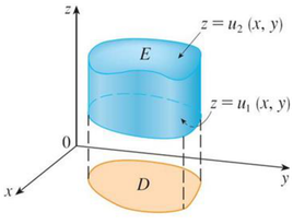
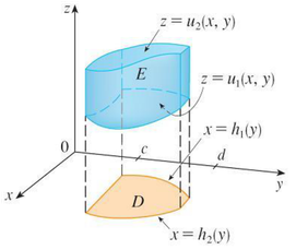
A solid region $E$ is said to be of type 1 if it lies between the graphs of two continuous functions of $x$ and $y$ that is:

$E = \{(x, y, z) \mid (x, y) \in D,\ u_1(x, y) \le z \le u_2(x, y)\} \qquad \ldots (25)$

where $D$ is the projection of $E$ onto the $xy$-plane as shown in Figure 10.25.

Figure 10.25: A type I solid region

Notice that the upper boundary of the solid $E$ is the surface with equation $z = u_2(x, y)$, while the lower boundary is the surface $z = u_1(x, y)$. By the same sort of argument, it can be shown that if $E$ is a type 1 region given by Eq. (25), then

$\iiint_E f(x, y, z)\,dV = \iint_D\left[\int_{u_1(x, y)}^{u_2(x, y)} f(x, y, z)\,dz\right]dA \qquad \ldots (26)$

The meaning of the inner integral on the right side of Eq. (26) is that $x$ and $y$ are held fixed, and therefore $u_1(x, y)$ and $u_2(x, y)$ are regarded as constants, while $f(x, y, z)$ is integrated with respect to $z$.

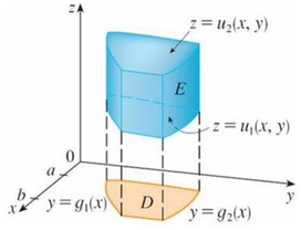
In particular, if the projection $D$ of $E$ onto the $xy$-plane is a type I plane region (as in Figure 10.26).

Figure 10.26: A type I solid region where the projection D is a type I plane region

Then

$E = \{(x, y, z) \mid a \le x \le b,\ g_1(x) \le y \le g_2(x),\ u_1(x, y) \le z \le u_2(x, y)\}$

and Eq. (26) becomes:

$\iiint_E f(x, y, z)\,dV = \int_a^b\int_{g_1(x)}^{g_2(x)}\int_{u_1(x, y)}^{u_2(x, y)} f(x, y, z)\,dz\,dy\,dx \qquad \ldots (27)$

If, on the other hand, $D$ is a type II plane region (as in Figure 10.27), then

$E = \{(x, y, z) \mid c \le y \le d,\ h_1(y) \le x \le h_2(y),\ u_1(x, y) \le z \le u_2(x, y)\}$

and Eq. (26) becomes:

$\iiint_E f(x, y, z)\,dV = \int_c^d\int_{h_1(y)}^{h_2(y)}\int_{u_1(x, y)}^{u_2(x, y)} f(x, y, z)\,dz\,dx\,dy \qquad \ldots (28)$

Figure 10.27: A type I solid region with type II projection

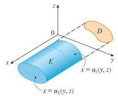
A solid region $E$ is of type 2 if it is of the form:

$E = \{(x, y, z) \mid (y, z) \in D,\ u_1(y, z) \le x \le u_2(y, z)\}$

where, this time, $D$ is the projection of $E$ onto the $yz$-plane (see Figure 10.28).

Figure 10.28: A type II region

The back surface is $x = u_1(y, z)$, the front surface is $x = u_2(y, z)$, and we have:

$\iiint_E f(x, y, z)\,dV = \iint_D\left[\int_{u_1(y, z)}^{u_2(y, z)} f(x, y, z)\,dx\right]dA \qquad \ldots (29)$

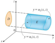
Finally, a type 3 region is of the form:

$E = \{(x, y, z) \mid (x, z) \in D,\ u_1(x, z) \le y \le u_2(x, z)\}$

where $D$ is the projection of $E$ onto the $xz$-plane, $y = u_1(x, z)$ is the left surface, and $y = u_2(x, z)$ is the right surface (see Figure 10.29).

Figure 10.29: A type III region

For this type of region we have:

$\iiint_E f(x, y, z)\,dV = \iint_D\left[\int_{u_1(x, z)}^{u_2(x, z)} f(x, y, z)\,dy\right]dA \qquad \ldots (30)$

In each of Eq. (29) and (30) there may be two possible expressions for the integral depending on whether $D$ is a type I or type II plane region (and corresponding to Eq. (27) and (28)).

Example 10.5

Evaluate

$\iiint_U xy^2z^3\,dx\,dy\,dz$

where the region $U$ (Figure 10.30) is bounded by the surfaces $z = xy$, $y = x$, $x = 0$, $x = 1$, $z = 0$.

Figure 10.30

Solution

The projection of the solid region $U$ onto the $xy$-plane looks as shown in Figure 10.31. Taking this into account, we find the corresponding iterated integral:

Figure 10.31

$$\begin{aligned} I = \iiint_U xy^2z^3\,dx\,dy\,dz &= \int_0^1 dx\int_0^x dy\int_0^{xy} xy^2z^3\,dz \\ \int_0^1 dx\int_0^x dy\left[\left(\frac{xy^2z^4}{4}\right)\bigg|_{z=0}^{z=xy}\right] &= \int_0^1 dx\int_0^x \left(xy^2\frac{x^4y^4}{4}\right)dy \\ &= \frac{1}{4}\int_0^1 dx\int_0^x x^5y^6\,dy = \frac{1}{4}\int_0^1 dx\left[\left(\frac{x^5y^7}{7}\right)\bigg|_{y=0}^{y=x}\right] \\ &= \frac{1}{4}\int_0^1 x^5\frac{x^7}{7}\,dx = \frac{1}{28}\int_0^1 x^{12}\,dx = \frac{1}{28}\left(\frac{x^{13}}{13}\right)\bigg|_0^1 = \frac{1}{28}\cdot\frac{1}{13} \\ &= \frac{1}{364} \end{aligned}$$

10.3.2 Application of Triple Integral

Triple or volume integral has important real-world application which can be applied in various scientific and engineering matters. In this section, we will discuss some of the application examples.

The most obvious usage of triple integral is to find the volume of a space confined within 3 dimensional boundary.

Example 10.6

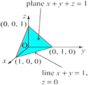
Find the volume of the tetrahedron defined by $x \ge 0$, $y \ge 0$, $z \ge 0$ and $x + y + z \le 1$.

Solution

Figure 10.32

For the tetrahedron shown above, its volume is:

$$\begin{aligned} V &= \int_{x=0}^{x=1}\int_{y=0}^{y=1}\int_{z=0}^{z=1-x-y} 1\,dz\,dy\,dx \\ &= \int_{x=0}^{x=1}\int_{y=0}^{y=1-x}(1 - x - y)\,dy\,dx \\ &= \int_{x=0}^{x=1}\frac{1}{2}(1 - x)^2\,dx = \frac{1}{6} \end{aligned}$$

---

10.4 Finding Mass and Center of Mass

Here, we will explore on how to find the mass, center of mass and moments of inertia using double integrals for a lamina (flat plate) and triple integrals for a three dimensional object with variable density. The density is generally considered to be a constant number when the lamina or the object is homogeneous; that is, the object has uniform density.

Refer to moments and centers of mass for the definitions and the methods of single integration to find the center of mass of a one dimensional object (for example, a thin rod). We are going to use a similar idea here except that the object is a two-dimensional lamina and thus, we use a double integral.

For a constant density function, then $\bar{x} = \dfrac{M_y}{m}$ and $\bar{y} = \dfrac{M_x}{m}$ give the centroid of the lamina.

10.4.1 Mass

Suppose that the lamina occupies a region $R$ in the $xy$-plane and let $\rho(x, y)$ be its density (in units of mass per unit area) at any point $(x, y)$. Hence:

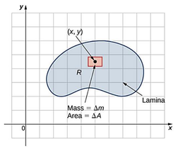
$\rho(x, y) = \lim_{\Delta A \to 0}\frac{\Delta m}{\Delta A}$

where $\Delta m$ and $\Delta A$ are the mass and area of a small rectangle containing the point $(x, y)$ and the limit is taken as the dimensions of the rectangle go to 0 (see Figure 10.33)

Figure 10.33: The density of a lamina at a point is the limit of its mass per area in a small rectangle about the point as the area goes to zero (0).

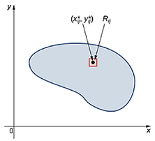
We divide the region $R$ into tiny rectangles $R_{ij}$ with area $\Delta A$ and choose $(x_{ij}^*, y_{ij}^*)$ as sample points. Then the mass $m_{ij}$ of each $R_{ij}$ is equal to $\rho(x_{ij}^*, y_{ij}^*)\Delta A$ (Figure 10.34). Let $a$ and $b$ be the number of subintervals in $x$ and $y$ respectively. Note that the shape might not always be rectangular.

Figure 10.34: Subdividing the lamina into small rectangle Rij each containing a sample point

The mass of the lamina:

$m = \lim_{k, l \to \infty}\sum_{i=1}^{a}\sum_{j=1}^{b} m_{ij} = \lim_{a, b \to \infty}\sum_{i=1}^{a}\sum_{j=1}^{b} \rho(x_{ij}^*, y_{ij}^*)\Delta A = \iint_R \rho(x, y)\,dA$

Example 10.7

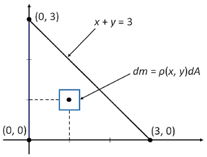
For a triangular lamina $R$ with vertices $(0, 0)$, $(0, 3)$, $(3, 0)$ and with density $\rho(x, y) = xy$ kg/m², find the total mass.

Solution

Figure 10.35: A lamina in the xy-plane with density ρ(x,y) = xy

We can find mass, $m$ using:

$$\begin{aligned} m &= \iint_R dm = \iint_R \rho(x, y)\,dA \\ &= \int_{x=0}^{x=3}\int_{y=0}^{y=3-x} xy\,dy\,dx = \int_{x=0}^{x=3}\left[x\frac{y^2}{2}\bigg|_{y=0}^{y=3-x}\right]dx = \int_{x=0}^{x=3}\frac{1}{2}x(3 - x)^2\,dx \\ &= \left[\frac{9x^2}{4} - x^3 + \frac{x^4}{8}\right]_{x=0}^{x=3} = \frac{27}{8} \end{aligned}$$

The mass, $m = \dfrac{27}{8}$ kg

On the other hand, for a mass of a matter bounded by $V$ with density of $\rho(x, y, z)$ at point $(x, y, z)$ can be calculated as $m = \iiint \rho(x, y, z)\,dz\,dy\,dx$ (or $\int_V \rho(x, y, z)\,dV$ (with appropriate limits)).

Example 10.8

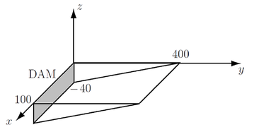
Figure 10.36: Water reservoir

A water reservoir shown above has the width of $x = 100$ m, length of $y = 400$ m, and the depth of the reservoir is given by $z = 40 - y/10$ m.

The density of the water can be approximated by $\rho(z) = a - b \times z$ where $a = 998$ kg m⁻³ and $b = 0.05$ kg m⁻⁴ i.e. at the surface ($z = 0$) the water has density $998$ kg m⁻³ (corresponding to a temperature of 20 °C while 40 m down i.e. $z = -40$, the water has a density of $1000$ kg m⁻³ (corresponding to the lower temperature of 4 °C. Find the total mass of water in the reservoir.

Solution

The mass of water in the reservoir is given by the integral of the function $\rho(z) = a - b \times z$. For each value of $x$ and $y$, the limits on $z$ will be from $y/10 - 40$ (bottom) to 0 (top). Limits on $y$ will be 0 to 400 m while the limits of $x$ will be 0 to 100 m. The mass of water is therefore given by the integral:

$m = \int_{x=0}^{100}\int_{y=0}^{400}\int_{z=y/10-40}^{0} (a - bz)\,dz\,dy\,dx$

This can be solved as follow:

$$\begin{aligned} m &= \int_{x=0}^{100}\int_{y=0}^{400}\left[az - \frac{b}{2}z^2\right]_{z=y/10-40}^{0} dy\,dx \\ &= \int_{x=0}^{100}\int_{y=0}^{400}\left[0 - a\left(\frac{y}{10} - 40\right) + \frac{b}{2}\left(\frac{y}{10} - 40\right)^2\right]dy\,dx \\ &= \int_{x=0}^{100}\int_{y=0}^{400}\left[40a - \frac{a}{10}y + \frac{b}{200}y^2 - 4by + 800b\right]dy\,dx \end{aligned}$$$$\begin{aligned} &= \int_{x=0}^{100}\left[40ay - \frac{a}{10}y^2 + \frac{b}{600}y^3 - 2by^2 + 800by\right]_{y=0}^{400}dx \\ &= \int_{x=0}^{100}\left(16000a - 8000a + \frac{320000}{3}b - 320000b + 320000b\right)dx \\ &= \int_{x=0}^{100}\left(8000a + \frac{320000}{3}b\right)dx = \left[8000ax + \frac{320000}{3}bx\right]_{x=0}^{100} \\ &= 8 \times 10^5 a + \frac{3.2}{3}\times 10^7 b = 7.984 \times 10^8 + \frac{0.16}{3}\times 10^7 \\ &= 7.989 \times 10^8\ \text{kg} \end{aligned}$$

So the mass ($m$) of water in the reservoir is $7.989 \times 10^8$ kg.

10.4.2 Center of Mass

Now that we have the expression for mass, we can find moments and centers of mass in two dimensions. The moment $M_x$ about the $x$-axis for $R$ is the limit of the sums of moments of the regions $R_{ij}$ about the $x$-axis. Hence:

$M_x = \lim_{k, l \to \infty}\sum_{i=1}^{a}\sum_{j=1}^{b}(y_{ij}^*)m_{ij} = \lim_{a, b \to \infty}\sum_{i=1}^{a}\sum_{j=1}^{b}(y_{ij}^*)\rho(x_{ij}^*y_{ij}^*)\Delta A = \iint_R y\rho(x, y)\,dA$

Similarly, the moment $M_y$ about the $y$-axis for $R$ is the limit of the sums of moments of the regions $R_{ij}$ about $y$-axis. Hence:

$M_y = \lim_{a, b \to \infty}\sum_{i=1}^{a}\sum_{j=1}^{b}(x_{ij}^*)m_{ij} = \lim_{a, b \to \infty}\sum_{i=1}^{a}\sum_{j=1}^{b}(x_{ij}^*)\rho(x_{ij}^*y_{ij}^*)\Delta A = \iint_R x\rho(x, y)\,dA$

To find the center of mass $(\bar{x}, \bar{y})$, the following expressions can be used:

$\bar{x} = \frac{M_y}{m} = \frac{\iint_R \rho(x, y)x\,dA}{\iint_R \rho(x, y)\,dA} \qquad \text{and} \qquad \bar{y} = \frac{M_x}{m} = \frac{\iint_R \rho(x, y)y\,dA}{\iint_R \rho(x, y)\,dA}$

Example 10.9

Consider the same triangular region $R$ (as in Example 10.7) with vertices $(0, 0)$, $(0, 3)$, $(3, 0)$ and with density $\rho(x, y) = xy$ kg/m².

Find center of mass.

Solution

Using the formula,

$\bar{x} = \frac{M_y}{m} = \frac{\iint_R \rho(x, y)x\,dA}{\iint_R \rho(x, y)\,dA} = \frac{81/20}{27/8} = \frac{6}{5}$

$\bar{y} = \frac{M_x}{m} = \frac{\iint_R \rho(x, y)y\,dA}{\iint_R \rho(x, y)\,dA} = \frac{81/20}{27/8} = \frac{6}{5}$

Thus, the center of mass is $\left(\dfrac{6}{5}, \dfrac{6}{5}\right)$

For three dimension, the expressions for the center of mass $(\bar{x}, \bar{y}, \bar{z})$ of a solid of density $\rho(x, y, z)$ are given below:

$\bar{x} = \frac{\int \rho(x, y, z)x\,dV}{\int \rho(x, y, z)\,dV}$

$\bar{y} = \frac{\int \rho(x, y, z)y\,dV}{\int \rho(x, y, z)\,dV}$

$\bar{z} = \frac{\int \rho(x, y, z)z\,dV}{\int \rho(x, y, z)\,dV}$

If $\rho$ does not vary with position, these simplify to:

$\bar{x} = \frac{\int x\,dV}{\int dV} \qquad \bar{y} = \frac{\int y\,dV}{\int dV} \qquad \bar{z} = \frac{\int z\,dV}{\int dV}$

Example 10.10

A uniform tetrahedron is enclosed by the planes $x = 0$, $y = 0$, $z = 0$ and $x + y + z = 4$. Find the volume and the position of the center of mass.

Solution

The volume integral of tetrahedron

$$\begin{aligned} V &= \int_{x=0}^{4}\int_{y=0}^{4-x}\int_{z=0}^{4-x-y} 1\,dz\,dy\,dx \\ &= \int_{x=0}^{4}\int_{y=0}^{4-x}\left[z\right]_{z=0}^{4-x-y} dy\,dx = \int_{x=0}^{4}\int_{y=0}^{4-x}(4 - x - y)\,dy\,dx \\ &= \int_{x=0}^{4}\left[4y - xy - \frac{1}{2}y^2\right]_{y=0}^{4-x} dx = \int_{x=0}^{4}\left[8 - 4x + \frac{1}{2}x^2\right]dx \\ &= \left[8x - 2x^2 + \frac{1}{6}x^3\right]_{x=0}^{4} = 32 - 32 + \frac{64}{6} = \frac{32}{3}. \end{aligned}$$

Then, we calculate $\int x\,dV$ as follows:

$$\begin{aligned} \int x\,dV &= \int_{x=0}^{4}\int_{y=0}^{4-x}\int_{z=0}^{4-x-y} x\,dz\,dy\,dx \\ &= \int_{x=0}^{4}\int_{y=0}^{4-x}\left[xz\right]_{z=0}^{4-x-y} dy\,dx = \int_{x=0}^{4}\int_{y=0}^{4-x}\left[x(4 - x - y) - 0\right]dy\,dx \\ &= \int_{x=0}^{4}\left[4xy - x^2y - \frac{1}{2}xy^2\right]_{y=0}^{4-x} dx = \int_{x=0}^{4}\left[8x - 4x^2 + \frac{1}{2}x^3\right]dx \\ &= \left[4x^2 - \frac{4}{3}x^3 + \frac{1}{8}x^4\right]_0^4 = 64 - \frac{256}{3} + 32 = \frac{32}{3} \end{aligned}$$

Thus, $\bar{x} = \dfrac{\int x\,dV}{\int dV} = \dfrac{32/3}{32/3} = 1$.

By symmetry (or by evaluating relevant integrals), it can be shown that $\bar{y} = \bar{z} = 1$ i.e. the center of mass is at $(1, 1, 1)$.

Example 10.11

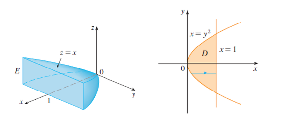
Find the center of mass of a solid of constant density that is bounded by the parabolic cylinder $x = y^2$ and the planes $x = z$, $z = 0$, and $x = 1$.

Solution

The solid $E$ and its projection onto the $xy$-plane are shown in Figure 10.37.

Figure 10.37

The lower and upper surfaces of $E$ are the planes $z = 0$ and $z = x$, so we describe $E$ as a type 1 region:

$E = \{(x, y, z) \mid -1 \le y \le 1,\ y^2 \le x \le 1,\ 0 \le z \le x\}$

Then, if the density is $\rho(x, y, z) = \rho$, the mass is:

$$\begin{aligned} m &= \iiint_E \rho\,dV = \int_{-1}^1\int_{y^2}^1\int_0^x \rho\,dz\,dx\,dy \\ &= \rho\int_{-1}^1\int_{y^2}^1 x\,dx\,dy = \rho\int_{-1}^1\left[\frac{x^2}{2}\right]_{x=y^2}^{x=1} dy \\ &= \frac{\rho}{2}\int_{-1}^1(1 - y^4)\,dy = \rho\int_0^1(1 - y^4)\,dy \\ &= \rho\left[y - \frac{y^5}{5}\right]_0^1 = \frac{4\rho}{5} \end{aligned}$$

Because of the symmetry of $E$ and $\rho$ about the $xz$-plane, we can immediately say that $M_{xz} = 0$ and therefore $\bar{y} = 0$. The other moments are:

$$\begin{aligned} M_{yz} &= \iiint_E x\rho\,dV = \int_{-1}^1\int_{y^2}^1\int_0^x x\rho\,dz\,dx\,dy \\ &= \rho\int_{-1}^1\int_{y^2}^1 x^2\,dx\,dy = \rho\int_{-1}^1\left[\frac{x^3}{3}\right]_{x=y^2}^{x=1} dy \\ &= \frac{2\rho}{3}\int_0^1(1 - y^6)\,dy = \frac{2\rho}{3}\left[y - \frac{y^7}{7}\right]_0^1 = \frac{4\rho}{7} \end{aligned}$$$$\begin{aligned} M_{xy} &= \iiint_E z\rho\,dV = \int_{-1}^1\int_{y^2}^1\int_0^x z\rho\,dz\,dx\,dy \\ &= \rho\int_{-1}^1\int_{y^2}^1\left[\frac{z^2}{2}\right]_{z=0}^{z=x} dx\,dy = \frac{\rho}{2}\int_{-1}^1\int_{y^2}^1 x^2\,dx\,dy \\ &= \frac{\rho}{3}\int_0^1(1 - y^6)\,dy = \frac{2\rho}{7} \end{aligned}$$

Therefore, the center of mass is:

$(\bar{x}, \bar{y}, \bar{z}) = \left(\frac{M_{yz}}{m}, \frac{M_{xz}}{m}, \frac{M_{xy}}{m}\right) = \left(\frac{5}{7}, 0, \frac{5}{14}\right)$

10.4.3 Moment of Inertia

The moment of inertia $I$ of a small particle of mass $m$ is defined as

$I = \text{Mass} \times \text{Distance}^2 \text{ or } I = md^2$

where $d$ is the perpendicular distance from the particle to the axis.

This concept is extended to a lamina with density function $\rho(x, y)$ and occupying a region $D$ by proceeding as we did for ordinary moments. We divide $D$ into small rectangles, approximate the moment of inertia of each subrectangle about the $x$-axis, and take the limit of the sum as the number of subrectangles becomes large. The result is the moment of inertia of the lamina about the x-axis:

$I_x = \lim_{m, n \to \infty}\sum_{i=1}^{m}\sum_{j=1}^{n}(y_{ij}^*)^2\rho(x_{ij}^*, y_{ij}^*)\Delta A = \iint_D y^2\rho(x, y)\,dA \qquad \ldots (31)$

Similarly, the moment of inertia about the y-axis is:

$I_y = \lim_{m, n \to \infty}\sum_{i=1}^{m}\sum_{j=1}^{n}(x_{ij}^*)^2\rho(x_{ij}^*, y_{ij}^*)\Delta A = \iint_D x^2\rho(x, y)\,dA \qquad \ldots (32)$

It is also of interest to consider the moment of inertia about the origin, also called the polar moment of inertia:

$I_0 = \lim_{m, n \to \infty}\sum_{i=1}^{m}\sum_{j=1}^{n}\left[(x_{ij}^*)^2 + (y_{ij}^*)^2\right]\rho(x_{ij}^*, y_{ij}^*)\Delta A = \iint_D (x^2 + y^2)\rho(x, y)\,dA \qquad \ldots (33)$

Note that $I_0 = I_x + I_y$

Example 10.12

Find the moments of inertia for the triangular region $R$ with vertices $(0, 0)$, $(2, 2)$ and $(2, 0)$ and with density $\rho(x, y) = xy$.

Solution

Using the expressions for the moments of inertia,

$I_x = \iint_R y^2\rho(x, y)\,dA = \int_{x=0}^{x=2}\int_{y=0}^{y=x} xy^3\,dy\,dx = \frac{8}{3}$

$I_y = \iint_R x^2\rho(x, y)\,dA = \int_{x=0}^{x=2}\int_{y=0}^{y=x} x^3y\,dy\,dx = \frac{16}{3}$

$I_0 = \iint_R (x^2 + y^2)\rho(x, y)\,dA = \int_0^2\int_{y=0}^{y=x}(x^2 + y^2)xy\,dy\,dx = I_x + I_y = 8$

To find the Moment of Inertia of a larger object, it is required to do a volume integration over all such particles. This will be covered in the following week.