Lecture 12: Line Integrals

Download the original PDF →

---

12.1 Introduction

Since in evaluating line integral we need to express the curve in parametric equation as function of $t$, let recognize parametric representation first.

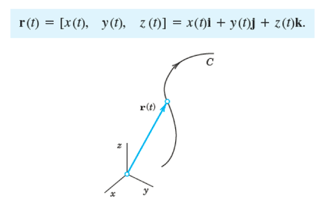
Bodies that move in space form paths that may be represented by curves $C$. This and other applications show the need for parametric representations of $C$ with parameter $t$, which may denote time or something else (see Fig. 12.1). A typical parametric representation is given by

$\mathbf{r}(t) = [x(t), \quad y(t), \quad z(t)] = x(t)\mathbf{i} + y(t)\mathbf{j} + z(t)\mathbf{k}.$

Figure 12.1: Parametric representation of curve

Here $t$ is the parameter and $x$, $y$, $z$ are Cartesian coordinates, that is, the usual rectangular coordinates. To each value $t = t_o$, there corresponds a point of $C$ with position vector $r(t_o)$ whose coordinates are $x(t_o), y(t_o), z(t_o)$.

When we give parametric equations and a parameter interval for a curve, we say that we have parametrized the curve. The equations and interval together constitute a parametrization of the curve. A given curve can be represented by different sets of parametric equations.

The advantages of using parametric representation are that, the coordinates $x$, $y$, $z$ all play an equal role, that is, all three coordinates are dependent variables. Moreover, the parametric representation induces an orientation on $C$. This means that as we increase $t$, we travel along the curve $C$ in a certain direction. The sense of increasing $t$ is called the positive sense on $C$. The sense of decreasing $t$ is then called the negative sense on $C$.

Table 12.1: Parametric Equation for Some Basic Curves

Curve	Counter-Clockwise	Clockwise *
$\dfrac{x^2}{a^2} + \dfrac{y^2}{b^2} = 1$ (Ellipse)	$x = a\cos(t)$ $y = b\sin(t)$ $0 \leq t \leq 2\pi$	$x = a\cos(t)$ $y = -b\sin(t)$ $0 \leq t \leq 2\pi$
$x^2 + y^2 = r^2$ (Circle)	$x = r\cos(t)$ $y = r\sin(t)$ $0 \leq t \leq 2\pi$	$x = r\cos(t)$ $y = -r\sin(t)$ $0 \leq t \leq 2\pi$
Line Segment from $(x_0, y_0, z_0)$ to $(x_1, y_1, z_1)$	$x = (1-t)x_0 + t x_1$ $y = (1-t)y_0 + t y_1$ $z = (1-t)z_0 + t z_1$ $0 \leq t \leq 1$
Parabola: $y = x^2$	Parabola: $x = t$, $y = t^2$, $-\infty \leq t \leq \infty$

* For clockwise curve, an alternative is to use the same counter-clockwise parameterization, but reverse the limits of integration. This gives a negative integral as compared to the counter-clockwise curve.

Example 12.1: Circle. Parametric Representation. Positive Sense

The circle $x^2 + y^2 = 4$, $z = 0$ in the $xy$-plane with center 0 and radius 2 can be represented parametrically by

$\mathbf{r}(t) = [2\cos t, 2\sin t, 0] \qquad \text{or simply by} \qquad \mathbf{r}(t) = [2\cos t, 2\sin t]$

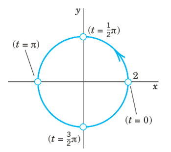
where $0 \leq t \leq 2\pi$. Indeed, $x^2 + y^2 = (2\cos t)^2 + (2\sin t)^2 = 4(\cos^2 t + \sin^2 t) = 4$. For $t = 0$ we have $\mathbf{r}(0) = [2, 0]$, for $t = \frac{1}{2}\pi$ we get $\mathbf{r}(\frac{1}{2}\pi) = [0, 2]$, and so on. The positive sense induced by this representation is the counterclockwise sense.

If we replace $t$ with $t^* = -t$, we have $t = -t^*$ and get

$\mathbf{r}^*(t^*) = [2\cos(-t^*), 2\sin(-t^*)] = [2\cos t^*, -2\sin t^*].$

This has reversed the orientation, and the circle is now oriented clockwise.

---

12.2 Basic Concepts

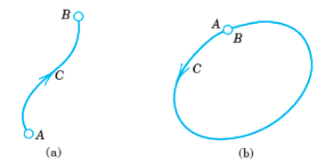
In a line integral, we shall integrate a given function, also called the integrand, along a curve $C$ in space or in the plane as shown in Figure 12.2. (Hence curve integral would be a better name but line integral is standard.)

Figure 12.2: Oriented curves

This requires that we represent the curve $C$ by a parametric representation

$\mathbf{r}(t) = [x(t), y(t), z(t)] = x(t)\mathbf{i} + y(t)\mathbf{j} + z(t)\mathbf{k} \qquad (a \leq t \leq b). \qquad (1)$

The curve $C$ is called the path of integration. Look at Fig. 12.2a. The path of integration goes from $A$ to $B$. Thus $A: \mathbf{r}(a)$ is its initial point and $B: \mathbf{r}(b)$ is its terminal point. $C$ is now oriented. The direction from $A$ to $B$, in which $t$ increases is called the positive direction on $C$. We mark it by an arrow. The points $A$ and $B$ may coincide, as it happens in Fig. 12.2b. Then $C$ is called a closed path.

A line integral of a vector function $F(r)$ over a curve $C: \mathbf{r}(t)$ is defined by

$\int_C \mathbf{F}(\mathbf{r}) \cdot d\mathbf{r} = \int_a^b \mathbf{F}(\mathbf{r}(t)) \cdot \mathbf{r}'(t)\, dt \qquad (2)$

Where $\mathbf{r}' = \dfrac{d\mathbf{r}}{dt}$ and $\mathbf{r}(t)$ is the parametric representation of $C$ as given in (1). Writing (2) in terms of components, with $d\mathbf{r} = [dx, dy, dz]$ and $' = \dfrac{d}{dt}$, we get

$$\begin{aligned} \int_C \mathbf{F}(\mathbf{r}) \cdot d\mathbf{r} &= \int_C M\, dx + N\, dy + P\, dz \\ &= \int_a^b M\, x' + N\, y' + P\, z'\, dt \end{aligned}$$

Note that the integrand in (2) is a scalar, not a vector, because we take the dot product. Indeed, $\mathbf{F} \bullet \mathbf{r}' / |\mathbf{r}'|$ is the tangential component of $\mathbf{F}$. Line integrals arises naturally in mechanics, where they give the work done by a force $\mathbf{F}$ in a displacement along $C$. This will be explained in detail below. We may thus call the line integral (2) the work integral.

Evaluating the Line Integral of F = Mi + Nj + Pk along C: r(t) = g(t)i + h(t)j + k(t)k

1. Express the vector field $\mathbf{F}$ in terms of the parametrized curve $C$ as $\mathbf{F}(\mathbf{r}(t))$ by substituting the components $x = g(t)$, $y = h(t)$, $z = k(t)$ of $\mathbf{r}$ into the scalar components $M(x, y, z)$, $N(x, y, z)$, $P(x, y, z)$ of $\mathbf{F}$.
2. Find the derivative (velocity) vector $d\mathbf{r}/dt$.
3. Evaluate the line integral with respect to the parameter $t$, $a \leq t \leq b$, to obtain

$\int_C \mathbf{F} \cdot d\mathbf{r} = \int_a^b \mathbf{F}(\mathbf{r}(t)) \cdot \frac{d\mathbf{r}}{dt}\, dt.$

Example 12.2: Evaluation of a Line Integral in the Plane

Find the value of line integral when $F(r) = [-y, -xy] = -y\mathbf{i} - xy\mathbf{j}$ and $C$ is the circular arc from A to B.

Solution

We may represent $C$ by $\mathbf{r}(t) = [\cos t, \sin t] = \cos t\,\mathbf{i} + \sin t\,\mathbf{j}$, where $0 \leq t \leq \pi/2$. Then $x(t) = \cos t$, $y(t) = \sin t$, and

$\mathbf{F}(\mathbf{r}(t)) = -y(t)\mathbf{i} - x(t)y(t)\mathbf{j} = [-\sin t, -\cos t \sin t] = -\sin t\,\mathbf{i} - \cos t \sin t\,\mathbf{j}.$

By differentiation, $\mathbf{r}'(t) = [-\sin t, \cos t] = -\sin t\,\mathbf{i} + \cos t\,\mathbf{j}$, set $\cos t = u$ in the second term

$$\begin{aligned} \int_C \mathbf{F}(\mathbf{r}) \cdot d\mathbf{r} &= \int_0^{\pi/2} [-\sin t, -\cos t \sin t] \bullet [-\sin t, \cos t]\, dt = \int_0^{\pi/2} \left(\sin^2 t - \cos^2 t \sin t\right) dt \\ &= \int_0^{\pi/2} \frac{1}{2}(1 - \cos 2t)\, dt - \int_1^0 u^2(-du) = \frac{\pi}{4} - 0 - \frac{1}{3} \approx 0.4521. \end{aligned}$$

Example 12.3: Line Integral in Space

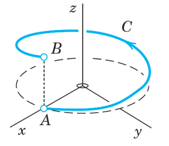
The evaluation of line integral in space is practically the same as it is in the plane. To see this, find the value of line integral when $F(r) = [z, x, y] = z\mathbf{i} + x\mathbf{j} + y\mathbf{k}$ and $C$ is the helix. Given that

$\mathbf{r}(t) = [\cos t, \sin t, 3t] = \cos t\,\mathbf{i} + \sin t\,\mathbf{j} + 3t\,\mathbf{k}$

Solution

From the parametrization above we have $x(t) = \cos t$, $y(t) = \sin t$, $z(t) = 3t$. Thus

$\mathbf{F}(\mathbf{r}(t)) \cdot \mathbf{r}'(t) = (3t\,\mathbf{i} + \cos t\,\mathbf{j} + \sin t\,\mathbf{k}) \bullet (-\sin t\,\mathbf{i} + \cos t\,\mathbf{j} + 3\mathbf{k}).$

The dot product is $3t(-\sin t) + \cos^2 t + 3 \sin t$. Hence

$\int_C \mathbf{F}(\mathbf{r}) \cdot d\mathbf{r} = \int_0^{2\pi} \left(-3t \sin t + \cos^2 t + 3 \sin t\right) dt = 6\pi + \pi + 0 = 7\pi \approx 21.99.$

Example 12.4: Evaluation of a Line Integral along the Curve, C

Evaluate $\displaystyle \int_c \mathbf{F} \cdot d\mathbf{r}$, where $F(x, y, z) = z\mathbf{i} + xy\,\mathbf{j} - y^2\mathbf{k}$ along the curve $C$ given by $\mathbf{r}(t) = t^2\mathbf{i} + t\mathbf{j} + \sqrt{t}\,\mathbf{k}$, $0 \leq t \leq 1$.

Solution

$\text{SOL} = \frac{17}{20}$

Simple general properties of the line integral (2)

$a) \quad \int_C k\mathbf{F} \cdot d\mathbf{r} = k\int_C \mathbf{F} \cdot d\mathbf{r} \qquad (k \text{ constant})$

$b) \quad \int_C (\mathbf{F} + \mathbf{G}) \cdot d\mathbf{r} = \int_C \mathbf{F} \cdot d\mathbf{r} + \int_C \mathbf{G} \cdot d\mathbf{r}$

$c) \quad \int_C \mathbf{F} \cdot d\mathbf{r} = \int_{C_1} \mathbf{F} \cdot d\mathbf{r} + \int_{C_2} \mathbf{F} \cdot d\mathbf{r}$

Figure 12.3 Formula (c)

where in (c) the path $C$ is subdivided into two arcs $C_1$ and $C_2$ that have the same orientation as $C$ (Fig. 12.3). In (b) the orientation of $C$ is the same in all three integrals. If the sense of integration along $C$ is reversed, the value of the integral is multiplied by -1.

---

12.3 Line Integral: Work Done by Force

Suppose that the vector field $\mathbf{F} = M(x, y, z)\mathbf{i} + N(x, y, z)\mathbf{j} + P(x, y, z)\mathbf{k}$ represents a force throughout a region in space (it might be the force of gravity or an electromagnetic force of some kind) and that

$\mathbf{r}(t) = g(t)\mathbf{i} + h(t)\mathbf{j} + k(t)\mathbf{k}, \qquad a \leq t \leq b,$

is a smooth curve in the region. For a curve $C$ in space, we define the work done by a continuous force field $\mathbf{F}$ to move an object along $C$ from a point $A$ to another point $B$ as follows.

DEFINITION

Let $C$ be a smooth curve parametrized by $\mathbf{r}(t)$, $a \leq t \leq b$, and $\mathbf{F}$ be a continuous force field over a region containing $C$. Then the work done in moving an object from the point $A = \mathbf{r}(a)$ to the point $B = \mathbf{r}(b)$ along $C$ is

$W = \int_C \mathbf{F} \cdot \mathbf{T}\, ds = \int_a^b \mathbf{F}(\mathbf{r}(t)) \cdot \frac{d\mathbf{r}}{dt}\, dt.$

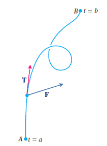
In other words, the work done by a force $F$ is the line integral of the scalar component $F.T$ over the smooth curve from $A$ to $B$ as shown in Fig 12.4. The sign of the number we calculate with this integral depends on the direction in which the curve is traversed. If we reverse the direction of motion, then we reverse the direction of $\mathbf{T}$ in Figure 12.4 and change the sign of $\mathbf{F} \cdot \mathbf{T}$ and its integral.

Figure 12.4: The work done by a force F is the line

Example 12.5

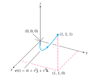
Find the work done by the force field $\mathbf{F} = (y - x^2)\mathbf{i} + (z - y^2)\mathbf{j} + (x - z^2)\mathbf{k}$ along the curve $\mathbf{r}(t) = t\mathbf{i} + t^2\mathbf{j} + t^3\mathbf{k}$, $0 \leq t \leq 1$, from $(0, 0, 0)$ to $(1, 1, 1)$

Solution

First we evaluate $\mathbf{F}$ on the curve $\mathbf{r}(t)$:

$$\begin{aligned} \mathbf{F} &= (y - x^2)\mathbf{i} + (z - y^2)\mathbf{j} + (x - z^2)\mathbf{k} \\ &= (\underbrace{t^2 - t^2}_{0})\mathbf{i} + (t^3 - t^4)\mathbf{j} + (t - t^6)\mathbf{k}. \qquad \text{Substitute } x = t, \ y = t^2, \ z = t^3. \end{aligned}$$

Then we find $d\mathbf{r}/dt$,

$\frac{d\mathbf{r}}{dt} = \frac{d}{dt}\left(t\mathbf{i} + t^2\mathbf{j} + t^3\mathbf{k}\right) = \mathbf{i} + 2t\mathbf{j} + 3t^2\mathbf{k}.$

Finally, we find $\mathbf{F} \cdot d\mathbf{r}/dt$ and integrate from $t = 0$ to $t = 1$:

$$\begin{aligned} \mathbf{F} \cdot \frac{d\mathbf{r}}{dt} &= \left[(t^3 - t^4)\mathbf{j} + (t - t^6)\mathbf{k}\right] \cdot \left(\mathbf{i} + 2t\mathbf{j} + 3t^2\mathbf{k}\right) \\ &= (t^3 - t^4)(2t) + (t - t^6)(3t^2) = 2t^4 - 2t^5 + 3t^3 - 3t^8 \end{aligned}$$

so,

$$\begin{aligned} \text{Work} &= \int_0^1 \left(2t^4 - 2t^5 + 3t^3 - 3t^8\right) dt \\ &= \left[\frac{2}{5}t^5 - \frac{2}{6}t^6 + \frac{3}{4}t^4 - \frac{3}{9}t^9\right]_0^1 = \frac{29}{60}. \end{aligned}$$

Example 12.6

Find the work done by the force fields $\mathbf{F} = x\mathbf{i} + y\mathbf{j} + z\mathbf{k}$ in moving an object along the curve $C$ parameterized by $\mathbf{r}(t) = \cos(\pi t)\,\mathbf{i} + t^2\mathbf{j} + \sin(\pi t)\,\mathbf{k}$, $0 \leq t \leq 1$

Solution

We begin by writing $\mathbf{F}$ along $C$ as a function of $t$,

$\mathbf{F}(\mathbf{r}(t)) = \cos(\pi t)\,\mathbf{i} + t^2\mathbf{j} + \sin(\pi t)\,\mathbf{k}.$

Next we compute $d\mathbf{r}/dt$,

$\frac{d\mathbf{r}}{dt} = -\pi \sin(\pi t)\,\mathbf{i} + 2t\mathbf{j} + \pi \cos(\pi t)\,\mathbf{k}.$

We then calculate the dot product,

$\mathbf{F}(\mathbf{r}(t)) \cdot \frac{d\mathbf{r}}{dt} = -\pi \sin(\pi t)\cos(\pi t) + 2t^3 + \pi \sin(\pi t)\cos(\pi t) = 2t^3.$

The work done is the line integral

$\int_a^b \mathbf{F}(\mathbf{r}(t)) \cdot \frac{d\mathbf{r}}{dt}\, dt = \int_0^1 2t^3\, dt = \left.\frac{t^4}{2}\right|_0^1 = \frac{1}{2}.$

Path Dependence

Path Dependence

The line integral generally depends not only on $\mathbf{F}$ and on the endpoints $A$ and $B$ of the path, but also on the path itself along which the integral is taken.

Take, for instance, the straight segment $C_1: r_1(t) = [t, t, 0]$ and the parabola $C_2: r_2(t) = [t, t^2, 0]$ as shown in Figure 12.5 with $0 \leq t \leq 1$ and integrate $F = [0, xy, 0]$. Then

For curve $C_1$: $r_1'(t) = [1, 1, 0]$, $F = [0, (t)(t), 0]$, therefore $F(r_1(t)) \bullet r_1'(t) = t^2$

For curve $C_2$: $r_2'(t) = [1, 2t, 0]$, $F = [0, (t)(t^2), 0]$, therefore $F(r_2(t)) \bullet r_2'(t) = 2t^4$

It is obvious that the two integrands of the line integral are different even though the two curves share the same endpoints A and B. Logically, this gives different values of 1/3 and 2/5 respectively.

Figure 12.5: Proof of Theorem

As an additional information, if a vector function $F$ is the gradient of a scalar function $F = \nabla f$, this vector function $F$ is known as a conservative vector field, and its line integral is interestingly independent on path, which means integrating $F$ along $C_1$ or $C_2$ produces the same value for the same endpoints A and B: $\int_{c_1} F \cdot dr_1 = \int_{c_2} F \cdot dr_2$

Example 12.7:

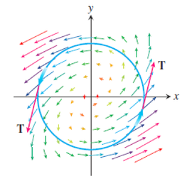
Evaluate the line integral with the vector function given as $F(x, y) = (x - y)\mathbf{i} + x\mathbf{j}$. The curve $C$ is a closed curve that forms a unit circle. A closed circular curve can be parameterized as below, considering a range of $t$ that forms the complete circular path:

$C: r(t) = \cos(t)\,\mathbf{i} + \sin(t)\,\mathbf{j}, \qquad 0 \leq t \leq 2\pi$

Solution

From $F(x, y) = (x - y)\mathbf{i} + x\mathbf{j}$ and $C: r(t) = \cos(t)\,\mathbf{i} + \sin(t)\,\mathbf{j}$, $0 \leq t \leq 2\pi$, we obtain:

$F(x, y) = (x - y)\mathbf{i} + x\mathbf{j}, \qquad \frac{d\mathbf{r}}{dt} = -\sin(t)\,\mathbf{i} + \cos(t)\,\mathbf{j}$

Therefore: $F \cdot \dfrac{d\mathbf{r}}{dt} = -\sin t \cos t + \sin^2 t + \cos^2 t = -\sin t \cos t + 1$

$$\begin{aligned} \int_0^{2\pi} (-\sin t)(\cos t) + 1\, dt &= \left[\frac{(\cos t)^2}{2} + t\right]_0^{2\pi} \\ &= \left(\frac{1}{2} + 2\pi\right) - \left(\frac{1}{2} + 0\right) \\ &= 2\pi \end{aligned}$$

Figure 12.6: The vector field has a counter clockwise circulation of 2π around the unit circle.

Example 12.8

Evaluate the closed-curve line integral

$\oint_C -y^2 dx + xy\, dy,$

Where $C$ is the square cut from the first quadrant by the lines $x = 1$ and $y = 1$ (counter-clockwise)

Solution

$\oint_C -y^2 dx + xy\, dy = \oint_{C_1}\left(-y^2\left(\frac{dx}{dt}\right) + xy\left(\frac{dy}{dt}\right)\right) dt + \cdots + \oint_{C_4}\left(-y^2\left(\frac{dx}{dt}\right) + xy\left(\frac{dy}{dt}\right)\right) dt :$

$C_1$: y=0, 0≤x≤1 (from 0 to 1)	Use x=t, y=0 $\dfrac{dx}{dt} = 1, \dfrac{dy}{dt} = 0$	$\int_0^1\left(-(0^2)(1) + (t)(0)(0)\right) dt = 0$
$C_2$: x=1, 0≤y≤1 (from 0 to 1)	Use x=1, y=t $\dfrac{dx}{dt} = 0, \dfrac{dy}{dt} = 1$	$\int_0^1\left(-(t^2)(0) + (1)(t)(1)\right) dt = \left[\dfrac{t^2}{2}\right]_0^1 = \dfrac{1}{2}$
$C_3$: y=1, 0≤x≤1 (from 1 to 0)	Use x=t, y=1 $\dfrac{dx}{dt} = 1, \dfrac{dy}{dt} = 0$	$\int_1^0\left(-(1^2)(1) + (t)(1)(0)\right) dt = -\int_0^1 -1\, dt = [t]_0^1 = 1$
$C_4$: x=0, 0≤y≤1 (from 1 to 0)	Use x=0, y=t $\dfrac{dx}{dt} = 0, \dfrac{dy}{dt} = 1$	$\int_0^1\left(-(t^2)(0) + (0)(t)(1)\right) dt = 0$

Therefore, $\displaystyle \oint_C -y^2 dx + xy\, dy = 0 + \frac{1}{2} + 1 + 0 = \frac{3}{2}$

Example 12.9

Compute $\oint xy\, dx + xy\, dy$, over the counter-clockwise rectangle with corners (1,1), (3,1), (3,2), (1,2).

Solution

$\oint_C xy\, dx + xy\, dy = \oint_{C_1}\left(xy\left(\frac{dx}{dt}\right) + xy\left(\frac{dy}{dt}\right)\right) dt + \cdots + \oint_{C_4}\left(xy\left(\frac{dx}{dt}\right) + xy\left(\frac{dy}{dt}\right)\right) dt$

$C_1$: y=1, 1≤x≤3 (from 1 to 3)	Use x=t, y=1 $\dfrac{dx}{dt} = 1, \dfrac{dy}{dt} = 0$	$\int_1^3\left((t)(1)(1) + (t)(1)(0)\right) dt$ $= \int_1^3 t\, dt = \dfrac{8}{2}$
$C_2$: x=3, 1≤y≤2 (from 1 to 2)	Use x=3, y=t $\dfrac{dx}{dt} = 0, \dfrac{dy}{dt} = 1$	$\int_1^2\left((3)(t)(0) + (3)(t)(1)\right) dt$ $= \int_1^2 3t\, dt = \dfrac{9}{2}$
$C_3$: y=2, 1≤x≤3 (from 3 to 1)	Use x=t, y=2 $\dfrac{dx}{dt} = 1, \dfrac{dy}{dt} = 0$	$\int_3^1\left((t)(2)(1) + (t)(2)(0)\right) dt$ $= -\int_1^3 2t\, dt = -\dfrac{16}{2}$
$C_4$: x=1, 1≤y≤2 (from 2 to 1)	Use x=1, y=t $\dfrac{dx}{dt} = 0, \dfrac{dy}{dt} = 1$	$\int_2^1\left((1)(t)(0) + (1)(t)(1)\right) dt$ $= -\int_1^2 t\, dt = -\dfrac{3}{2}$

$\oint xy\, dx + xy\, dy = \frac{8}{2} + \frac{9}{2} - \frac{16}{2} - \frac{3}{2} = -1$

The solutions of line integral involving closed curve can be tedious when the closed curve is defined by multiple sections as in Examples 12.8 and 12.9. In some cases, it will be more convenient to relate a closed-curve line integral with an integral involving the curl of the vector function $F$ over a surface that is bounded by the closed curve. This is known as the (circulation form of) Green's theorem, which is explained in the topic of Stokes' theorem.