Lecture 13: Surface Integrals

Download the original PDF →

---

13.1 Surfaces for Surface Integral

The idea that will lead to the concept of a surface integral is quite similar to that which led to a line integral. We say briefly 'surface' also for a portion of a surface, just as we said 'curve' for an arc of a curve, for simplicity. Representations of a surface $S$ in $xyz$-space are

$z = f(x,y) \qquad \text{or} \qquad g(x,y,z) = 0 \qquad (1)$

For example, $z = +\sqrt{a^2-x^2-y^2}$ or $x^2+y^2+z^2-a^2 = 0$ $(z \geq 0)$ represents hemisphere of radius $a$ and centre 0.

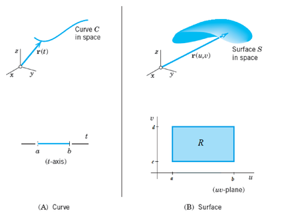
Now for curves $C$ in line integrals, it was more practical and gave greater flexibility to use a parametric representation $\mathbf{r} = \mathbf{r}(t)$ where $a \leq t \leq b$. This is a mapping of the interval $a \leq t \leq b$ located on the $t$-axis, onto the curve $C$ in the $xyz$-space. It maps every $t$ in that interval onto the point of $C$ with position vector $\mathbf{r}(t)$ (see Figure 13.1)

Figure 13.1: Parametric representations of a curve and a surface

Similarly, for surfaces $S$ in surface integrals, it will often be more practical to use a parametric representation. Surfaces are two-dimensional. Hence we need two parameters, which we call $u$ and $v$. Thus a parametric representation of a surface $S$ in space is of the form

$\mathbf{r}(u,v) = [x(u,v), y(u,v), z(u,v)] = x(u,v)\,\mathbf{i} + y(u,v)\,\mathbf{j} + z(u,v)\,\mathbf{k} \qquad (2)$

when $(u,v)$ varies in some region $R$ of the $uv$-plane. This mapping (2) maps every point $(u,v)$ in $R$ onto the point of $S$ with position vector $\mathbf{r}(u,v)$ (see Figure 13.1(B)).

Parametric Representation of a Cylinder

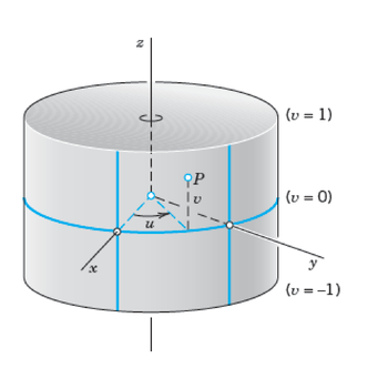
The circular cylinder $x^2+y^2 = a^2$, $-1 \leq z \leq 1$, has radius $a$, height 2, and the $z$-axis as axis. A parametric representation is

$\mathbf{r}(u,v) = [a\cos u, a\sin u, v] = a\cos u\,\mathbf{i} + a\sin u\,\mathbf{j} + v\,\mathbf{k} \qquad (3)$

The components of $\mathbf{r}$ are $x = a\cos u$, $y = a\sin u$, $z = v$. The parameters $u$, $v$ vary in the rectangle $R$: $0 \leq u \leq 2\pi$, $-1 \leq v \leq 1$ in the $uv$-plane. The curves $u = \text{const}$ are vertical straight lines. The curves $v = \text{const}$ are parallel circles. The point $P$ in Figure 13.2 corresponds to $u = \pi/3 = 60°$, $v = 0.7$.

Figure 13.2: Parametric representation of a cylinder

Parametric Representation of a Sphere

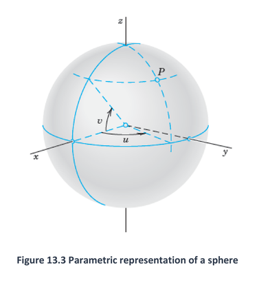
A sphere $x^2+y^2+z^2 = a^2$ can be represented in the form

$\mathbf{r}(u,v) = a\cos v\cos u\,\mathbf{i} + a\cos v\sin u\,\mathbf{j} + a\sin v\,\mathbf{k} \qquad (4)$

where the parameters $u$, $v$ vary in the rectangle $R$ in the $uv$-plane given by the inequalities $0 \leq u \leq 2\pi$, $-\pi/2 \leq v \leq \pi/2$. The components of $\mathbf{r}$ are

$x = a\cos v\cos u, \qquad y = a\cos v\sin u, \qquad z = a\sin v$

The curves $u = \text{const}$ and $v = \text{const}$ are the 'meridian' and 'parallels' on $S$ (as shown in Figure 13.3). This representation is used in geography for measuring the latitude and longitude of points on the globe. Another parametric representation of the sphere also used in mathematics is

$\mathbf{r}(u,v) = a\cos u\sin v\,\mathbf{i} + a\sin u\sin v\,\mathbf{j} + a\cos v\,\mathbf{k} \qquad (4^*)$

where $0 \leq u \leq 2\pi$, $0 \leq v \leq \pi$

Figure 13.3: Parametric representation of a sphere

Parametric Representation of a Cone

A circular cone $z = \sqrt{x^2+y^2}$, $0 \leq z \leq H$ can be represented by

$\mathbf{r}(u,v) = [u\cos v, u\sin v, u] = u\cos v\,\mathbf{i} + u\sin v\,\mathbf{j} + u\,\mathbf{k} \qquad (5)$

in components $x = u\cos v$, $y = u\sin v$, $z = u$. The parameters vary in the rectangle $R$: $0 \leq u \leq H$, $0 \leq v \leq 2\pi$

13.2 Surface Integral

The extension of the idea of an integral to line and double integrals are not the only generalization that can be made. We can also extend the idea to integration over a general surface, $S$. Two types of such integrals occur:

$\iint_S f(x,y,z)\,dS \qquad (6)$

Scalar field, e.g.: surface density

$\iint_S \mathbf{F}(\mathbf{r})\cdot\hat{\mathbf{n}}\,dS = \iint_S \mathbf{F}(\mathbf{r})\cdot d\mathbf{S} \qquad (7)$

Vector field, e.g.: fluid velocity

Note that $d\mathbf{S} = \hat{\mathbf{n}}\,dS$ is the vector element of area, where $\hat{\mathbf{n}}$ is the unit outward-drawn normal vector to the element $dS$.

13.2.1 Surface Integral of Vector Field

In general, the surface $S$ can be described in terms of two parameters, $u$ and $v$ say, so that on $S$

$\mathbf{r}(u,v) = [x(u,v), y(u,v), z(u,v)] = x(u,v)\,\mathbf{i} + y(u,v)\,\mathbf{j} + z(u,v)\,\mathbf{k}$

where $(u,v)$ varies over a region $R$ in the $uv$-plane. We assume $S$ to be piecewise smooth, so that $S$ has a normal vector

$\mathbf{N} = \mathbf{r}_u \times \mathbf{r}_v \qquad \text{and unit normal vector} \qquad \mathbf{n} = \frac{1}{|\mathbf{N}|}\mathbf{N}$

at every point (except perhaps for some edges or cusps, as for a cube or cone). For a given vector function $\mathbf{F}$ we can now define the surface integral over $S$ by

$\iint_S \mathbf{F}\cdot\mathbf{n}\,dS = \iint_R \mathbf{F}(\mathbf{r}(u,v))\cdot\mathbf{N}(u,v)\,du\,dv \qquad (8)$

Here $\mathbf{N} = |\mathbf{N}|\mathbf{n}$ by equation (12), and $|\mathbf{N}| = |\mathbf{r}_u \times \mathbf{r}_v|$ is the area of the parallelogram with sides $\mathbf{r}_u$ and $\mathbf{r}_v$, by the definition of cross product. Hence

$\mathbf{n}\,dS = \mathbf{n}|\mathbf{N}|\,du\,dv = \mathbf{N}\,du\,dv \qquad (8^*)$

and we see that $dS = |\mathbf{N}|\,du\,dv$ is the element of area of $S$.

also $\mathbf{F}\cdot\mathbf{n}$ is the normal component of $\mathbf{F}$. This integral arises naturally in flow problems, where it gives the flux across $S$ when $\mathbf{F} = \rho\mathbf{v}$. The flux across $S$ is the mass of fluid crossing $S$ per unit time. Furthermore, $\rho$ is the density of the fluid and $\mathbf{v}$ the velocity vector of the flow, as illustrated by Example 13.1 below. We may thus call the surface integral (8) the flux integral.

We can write (8) in components, using $\mathbf{F} = [F_1, F_2, F_3]$, $\mathbf{N} = [N_1, N_2, N_3]$, and $\mathbf{n} = [\cos\alpha, \cos\beta, \cos\gamma]$. Here $\alpha$, $\beta$, $\gamma$ are the angles between $\mathbf{n}$ and the coordinate axes; indeed, for the angle between $\mathbf{n}$ and $\mathbf{i}$.

$$\begin{aligned} \iint_S \mathbf{F}\cdot\mathbf{n}\,dS &= \iint_S (F_1\cos\alpha + F_2\cos\beta + F_3\cos\gamma)\,dS \qquad (9) \\ &= \iint_R (F_1N_1 + F_2N_2 + F_3N_3)\,du\,dv \end{aligned}$$

In (9) we can write $\cos\alpha\,dS = dydz$, $\cos\beta\,dS = dzdx$, $\cos\gamma\,dS = dxdy$. Then (9) becomes the following integral for the flux:

$\iint_S \mathbf{F}\cdot\mathbf{n}\,dS = \iint_S (F_1\,dydz + F_2\,dzdx + F_3\,dxdy) \qquad (10)$

We can use this formula to evaluate surface integrals by converting them to double integrals over regions in the coordinate planes of the xyz-coordinate system. But we must carefully take into account the orientation of $S$ (the choice of $\mathbf{n}$), as described in Section 13.3.1.

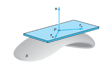
The tangent vectors of all the curves on a surface $S$ through a point $P$ of $S$ form a plane, called the tangent plane of $S$ at $P$ (refer to Figure 13.4). Exceptions are points where $S$ has an edge or a cusp (like a cone), so that $S$ cannot have a tangent plane at such a point. Furthermore, a vector perpendicular to the tangent plane is called a normal vector of $S$ at $P$.

Figure 13.4: Tangent plane and normal vector

Now since $S$ can be given by $\mathbf{r} = \mathbf{r}(u,v)$ in (2), the new idea is that we get a curve $C$ on $S$ by taking a pair of differentiable functions

$u = u(t), \qquad v = v(t)$

whose derivatives $u' = du/dt$ and $v' = dv/dt$ are continuous. Then $C$ has the position vector $\tilde{\mathbf{r}}(t) = \mathbf{r}(u(t), v(t))$. By differentiation and the use of the chain rule, we obtain a tangent vector of $C$ on $S$

$\tilde{\mathbf{r}}'(t) = \frac{d\tilde{\mathbf{r}}}{dt} = \frac{\partial\mathbf{r}}{\partial u}u' + \frac{\partial\mathbf{r}}{\partial v}v'$

Hence the partial derivatives $\mathbf{r}_u$ and $\mathbf{r}_v$ at $P$ are tangential to $S$ at $P$. We assume that they are linearly independent, which geometrically means that the curves $u = \text{const}$ and $v = \text{const}$ on $S$ intersect at $P$ at a non-zero angle. Then $\mathbf{r}_u$ and $\mathbf{r}_v$ span the tangent plane of $S$ at $P$. Hence their cross product gives a normal vector $\mathbf{N}$ of $S$ at $P$.

$\mathbf{N} = \mathbf{r}_u \times \mathbf{r}_v \neq 0 \qquad (11)$

The corresponding unit normal vector $\mathbf{n}$ of $S$ at $P$ is (Figure 13.4)

$\mathbf{n} = \frac{1}{|\mathbf{N}|}\mathbf{N} = \frac{1}{|\mathbf{r}_u \times \mathbf{r}_v|}\mathbf{r}_u \times \mathbf{r}_v \qquad (12)$

There is an alternative way of obtaining a unit normal vector of a surface $S$. If $S$ is represented by expression $g(x,y,z) = 0$, then, from prior knowledge that gradient of $g$ is always normal to $g$:

$\mathbf{n} = \frac{1}{|\operatorname{grad} g|}\operatorname{grad} g \qquad (12^*)$

Tangent Plane and Surface Normal

If a surface $S$ is given by (2) with continuous $\mathbf{r}_u = \dfrac{\partial\mathbf{r}}{\partial u}$ and $\mathbf{r}_v = \dfrac{\partial\mathbf{r}}{\partial v}$ at every point of $S$, then $S$ has, at every point $P$, a unique tangent plane passing through $P$ and spanned by $\mathbf{r}_u$ and $\mathbf{r}_v$ and a unique normal whose direction depends continuously on the points of $S$. A normal vector is given by (11) and the corresponding unit normal vector by (12) (see Figure 13.4).

Example 13.1

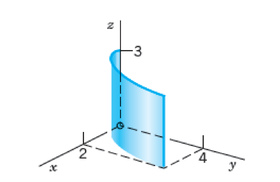
Compute the flux of water through the parabolic cylinder $S: y = x^2$, $0 \leq x \leq 2$, $0 \leq z \leq 3$ if the velocity vector is $\mathbf{v} = \mathbf{F} = [3z^2, 6, 6xz]$, speed being measured in meters/sec. (Generally, $\mathbf{F} = \rho\mathbf{v}$, but water has density $\rho = 1\ \text{g/cm}^3 = 1\ \text{ton/m}^3$)

Solution

Writing $x = u$ and $z = v$, we have $y = x^2 = u^2$. Hence a representation of $S$ is

$S: \quad \mathbf{r} = [u, u^2, v] \qquad (0 \leq u \leq 2, \ 0 \leq v \leq 3)$

By differentiation and by the definition of the cross product,

$\mathbf{N} = \mathbf{r}_u \times \mathbf{r}_v = [1, 2u, 0] \times [0, 0, 1] = [2u, -1, 0]$

On $S$, writing simply $\mathbf{F}(S)$ for $\mathbf{F}[\mathbf{r}(u,v)]$, we have $\mathbf{F}(S) = [3v^2, 6, 6uv]$. Hence $\mathbf{F}(S)\cdot\mathbf{N} = 6uv^2 - 6$. By integration we thus get from (7) the flux

$$\begin{aligned} \iint_S \mathbf{F}\cdot\mathbf{n}\,dS &= \int_0^3\int_0^2 (6uv^2 - 6)\,du\,dv = \int_0^3 \left[3u^2v^2 - 6u\right]_{u=0}^2 dv \\ &= \int_0^3 (12v^2 - 12)\,dv = \left[4v^3 - 12v\right]_{v=0}^3 = 108 - 36 = 72\ [\text{m}^3/\text{sec}] \end{aligned}$$

Or 72,000 liters/sec. Note that the $y$-component of $\mathbf{F}$ is positive (equal to 6), so that in figure above, the flow goes from left to right.

Example 13.2

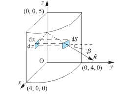
Compute the flux through the surface $S$, of the cylinder $x^2+y^2 = 16$ in the first octant between $z = 0$ and $z = 5$ if the velocity vector is $\mathbf{F} = [z, x, -3y^2z]$, that is, the flux $\displaystyle\iint_S \mathbf{F}\cdot d\mathbf{S}$.

Solution

Writing $x = u$ and $z = v$, we have $y = \sqrt{16-u^2}$ (from $x^2+y^2 = 16$)

$\mathbf{r}(u,v) = \left[u, \sqrt{16-u^2}, v\right]$

$\mathbf{r}_u = \frac{\partial\mathbf{r}}{\partial u} = \left[1, -\frac{u}{\sqrt{16-u^2}}, 0\right]$

$\mathbf{r}_v = \frac{\partial\mathbf{r}}{\partial v} = [0, 0, 1] \qquad \therefore \mathbf{N} = \mathbf{r}_v \times \mathbf{r}_u = \begin{vmatrix} \mathbf{i} & \mathbf{j} & \mathbf{k} \\ 0 & 0 & 1 \\ 1 & -\frac{u}{\sqrt{16-u^2}} & 0 \end{vmatrix} = \left[\frac{u}{\sqrt{16-u^2}}, 1, 0\right]$

$\mathbf{F}[\mathbf{r}(u,v)] = [v, u, -3(16-u^2)v]$

$\mathbf{F}[\mathbf{r}(u,v)]\cdot\mathbf{N} = \frac{uv}{\sqrt{16-u^2}} + u$

$\iint_S \mathbf{F}\cdot\mathbf{N}\,dS = \int_0^5\int_0^4 \frac{uv}{\sqrt{16-u^2}} + u\ du\,dv$

$$\begin{aligned} \therefore \int_0^5\left(v\left[\int_0^4 \frac{u}{\sqrt{16-u^2}}\,du\right] + \int_0^4 u\,du\right) &= \int_0^5\left[-\frac{v}{2}\int_0^4 \frac{-2u}{\sqrt{16-u^2}}\,du + \int_0^4 u\,du\right] dv \\ &= \int_0^5 -v\left[\sqrt{16-u^2}\right]_0^4 dv + \int_0^5\left[\frac{u^2}{2}\right]_0^4 dv \\ &= \int_0^5 4v\,dv + \int_0^5 8\,dv = 90 \end{aligned}$$

Comment: In this example, the solution shown uses a basic parameterization of $x = u$, $y = \sqrt{16-u^2}$, $z = v$, instead of the common cylindrical surface parameterization $x = 4\cos u$, $y = 4\sin u$, $z = v$ as learned earlier. Try to repeat this example using the cylindrical surface parameterization (Hint: integrals of the same field and the same surface should result in the same answer).

13.2.2 Surface Integral of Scalar Field

When the field (function) to be integrated is a scalar field, the resulted integral is known as the surface integral of a scalar field, or simply the scalar surface integral. So, $\iint_S f(x,y,z)\,dS$ has essentially the same concept as vector surface integral, but with a scalar field instead. Just as the vector surface integral, here, for a given surface $S$, suitable parameterization can be used: $x = x(u,v)$, $y = y(u,v)$, $z = z(u,v)$, which gives again the position vector $\mathbf{r}(u,v) = x(u,v)\mathbf{i} + y(u,v)\mathbf{j} + z(u,v)\mathbf{k}$.

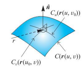
Just as the vector surface integral, the surface $S$ can be specified by a scalar point function $C(\mathbf{r}) = c$, where $c$ is a constant. Curves may be drawn on that surface, and in particular if we fix the value of one of the two parameters $u$ and $v$ then we obtain two families of curves. On one, $C_u(\mathbf{r}(u,v_0))$ the value of $u$ varies while $v$ is fixed, and on the other, $C_v(\mathbf{r}(u_0,v))$, the values of $v$ varies while $u$ is fixed, as shown in Figure 13.5. Then as indicated on Figure 13.5, the vector element of area $d\mathbf{S}$ is given by:

Figure 13.5: Parametric curves on a surface

$d\mathbf{S} = \frac{\partial\mathbf{r}}{\partial u}du \times \frac{\partial\mathbf{r}}{\partial v}dv = \frac{\partial\mathbf{r}}{\partial u} \times \frac{\partial\mathbf{r}}{\partial v} du\,dv$

$= \left(\frac{\partial x}{\partial u}, \frac{\partial y}{\partial u}, \frac{\partial z}{\partial u}\right) \times \left(\frac{\partial x}{\partial v}, \frac{\partial y}{\partial v}, \frac{\partial z}{\partial v}\right) du\,dv = (J_1\mathbf{i} + J_2\mathbf{j} + J_3\mathbf{k})\,du\,dv$

where

$J_1 = \frac{\partial y}{\partial u}\frac{\partial z}{\partial v} - \frac{\partial y}{\partial v}\frac{\partial z}{\partial u}, \qquad J_2 = \frac{\partial z}{\partial u}\frac{\partial x}{\partial v} - \frac{\partial z}{\partial v}\frac{\partial x}{\partial u}, \qquad J_3 = \frac{\partial x}{\partial u}\frac{\partial y}{\partial v} - \frac{\partial x}{\partial v}\frac{\partial y}{\partial u}$

However, instead of $d\mathbf{S} = \dfrac{\partial\mathbf{r}}{\partial u} \times \dfrac{\partial\mathbf{r}}{\partial v} du\,dv$, for scalar surface integral, we have:

$dS = \left|\frac{\partial\mathbf{r}}{\partial u} \times \frac{\partial\mathbf{r}}{\partial v}\right| du\,dv, \quad \text{where the magnitude} \left|\frac{\partial\mathbf{r}}{\partial u} \times \frac{\partial\mathbf{r}}{\partial v}\right| = \sqrt{J_1^2 + J_2^2 + J_3^2}$

$\iint_S f(x,y,z)\,dS = \iint_A f(u,v)\sqrt{J_1^2 + J_2^2 + J_3^2}\,du\,dv \qquad (13)$

Once the entire integral can be described with only $u$ and $v$, the integration can be carried out to obtain the value of the integral.

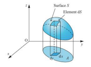
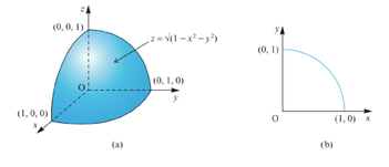
Sometimes, a given surface can be very clearly described by $z = z(x,y)$. A quick example is a vertical cone with $z = \sqrt{x^2+y^2}$. In this situation, we can simply adopt $x = u$, $y = v$ (and $z = \sqrt{u^2+v^2}$). In fact, we can directly write the two parameters as $x$ and $y$ without introducing new symbols $u$ and $v$. For example, if $z = z(x,y)$ describes a surface as in Figure 13.6, then

$\mathbf{r} = (x, y, z(x,y))$

with $x$ and $y$ as independent variables. Then, the cross product becomes:

$\frac{\partial\mathbf{r}}{\partial u} \times \frac{\partial\mathbf{r}}{\partial v} = \frac{\partial\mathbf{r}}{\partial x} \times \frac{\partial\mathbf{r}}{\partial y} = \left(-\frac{\partial z}{\partial x}\right)\mathbf{i} + \left(-\frac{\partial z}{\partial y}\right)\mathbf{j} + (1)\mathbf{k}$

$J_1 = -\frac{\partial z}{\partial x} \qquad J_2 = -\frac{\partial z}{\partial y} \qquad J_3 = 1$

Since $dS = \left|\dfrac{\partial\mathbf{r}}{\partial u} \times \dfrac{\partial\mathbf{r}}{\partial v}\right| du\,dv = \left|\dfrac{\partial\mathbf{r}}{\partial x} \times \dfrac{\partial\mathbf{r}}{\partial y}\right| dx\,dy$,

$\iint_S f(x,y,z)\,dS = \iint_R f(x,y,z(x,y))\sqrt{1 + \left(\frac{\partial z}{\partial x}\right)^2 + \left(\frac{\partial z}{\partial y}\right)^2}\,dx\,dy \qquad (14)$

Figure 13.6: A surface described by z = z(x, y)

Example 13.3

Evaluate the surface integral

$\iint_S (x + y + z)\,dS$

where $S$ is the portion of the sphere $x^2+y^2+z^2 = 1$ that lies in the first octant.

(a) Surface S (b) quadrant of a circle in the (x, y) plane

Solution

The surface $S$ is illustrated in the above figure. Taking

$z = \sqrt{1-x^2-y^2}$

we have

$\frac{\partial z}{\partial x} = \frac{-x}{\sqrt{1-x^2-y^2}}$

$\frac{\partial z}{\partial y} = \frac{-y}{\sqrt{1-x^2-y^2}}$

giving

$\sqrt{1 + \left(\frac{\partial z}{\partial x}\right)^2 + \left(\frac{\partial z}{\partial y}\right)^2} = \sqrt{\frac{x^2+y^2+(1-x^2-y^2)}{(1-x^2-y^2)}} = \frac{1}{\sqrt{1-x^2-y^2}}$

$\therefore \iint_S (x+y+z)\,dS = \iint_A \left[x + y + \sqrt{1-x^2-y^2}\right]\frac{1}{\sqrt{1-x^2-y^2}}\,dx\,dy$

where $A$ is the quadrant of a circle in the $(x,y)$ plane illustrated in Figure (b) (refer to the above Figure).

Thus,

$\iint_S (x+y+z)\,dS = \int_0^1\int_0^{\sqrt{1-x^2}} \left[\frac{x}{\sqrt{1-x^2-y^2}} + \frac{y}{\sqrt{1-x^2-y^2}} + 1\right] dy\,dx$

$$\begin{aligned} &= \int_0^1 \left[x\sin^{-1}\left(\frac{y}{\sqrt{1-x^2}}\right) - \sqrt{1-x^2-y^2} + y\right]_0^{\sqrt{1-x^2}} dx \\ &= \int_0^1 \left[\frac{\pi}{2}x + 2\sqrt{1-x^2}\right] dx = \left[\frac{\pi}{4}x^2 + x\sqrt{1-x^2} + \sin^{-1}x\right]_0^1 = \frac{3}{4}\pi \end{aligned}$$

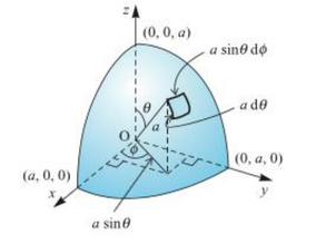
An alternative approach to evaluating the surface integral in this example is to evaluate it directly over the surface of the sphere using spherical polar coordinates. As illustrated in the Figure (c), on the surface of a sphere of radius $a$ we have,

$x = a\sin\theta\cos\phi, \quad y = a\sin\theta\sin\phi, \quad z = a\cos\theta, \quad dS = a^2\sin\theta\,d\theta\,d\phi$

(c) Surface element in spherical polar coordinates

The radius $a = 1$, so that

$\iint_S (x+y+z)\,dS = \int_0^{\pi/2}\int_0^{\pi/2}(\sin\theta\cos\phi + \sin\theta\sin\phi + \cos\theta)\sin\theta\,d\theta\,d\phi$

$= \int_0^{\pi/2}\left[\frac{1}{4}\pi\cos\phi + \frac{1}{4}\pi\sin\phi + \frac{1}{2}\right]d\phi = \frac{3}{4}\pi$

Example 13.4

Calculate the surface integral $\displaystyle\iint_S (x+y+z)\,dS$ where $S$ is the portion of the plane $x + 2y + 4z = 4$ lying in the first octant ($x \geq 0$, $y \geq 0$, $z \geq 0$)

Solution

Rewrite linear equation:

$z = \frac{4-x-2y}{4} = 1 - \frac{x}{4} - \frac{y}{2}$

$\frac{\partial z}{\partial x} = -\frac{1}{4} \qquad \frac{\partial z}{\partial y} = -\frac{1}{2}$

$\iint_S f(x,y,z)\,dS = \iint_A f(x,y,z(x,y))\sqrt{1 + \left(\frac{\partial z}{\partial x}\right)^2 + \left(\frac{\partial z}{\partial y}\right)^2}\,dx\,dy$

$\iint_S f(x,y,z)\,dS = \iint_A \left(x + y + 1 - \frac{x}{4} - \frac{y}{2}\right)\sqrt{1 + \left(-\frac{1}{4}\right)^2 + \left(-\frac{1}{2}\right)^2}\,dx\,dy$

$= \iint_A \left(\frac{3x}{4} + \frac{y}{2} + 1\right)\frac{\sqrt{21}}{4}\,dx\,dy$

$$\begin{aligned} &= \frac{\sqrt{21}}{4}\int_0^2\int_0^{4-2y}\left(\frac{3x}{4} + \frac{y}{2} + 1\right) dx\,dy = \frac{\sqrt{21}}{16}\int_0^2\left(\frac{3x^2}{2} + 2yx + 4x\right)_0^{4-2y} dy \\ &= \frac{\sqrt{21}}{32}\int_0^2\left(3(16-16y+4y^2) + 16y - 8y^2 + 32 - 16y\right) dy = \frac{\sqrt{21}}{32}\int_0^2 (80 - 48y + 4y^2)\,dy \\ &= \frac{\sqrt{21}}{8}\int_0^2 20 - 12y + y^2\,dy = \frac{\sqrt{21}}{8}\left[20y - 6y^2 + \frac{y^3}{3}\right]_0^2 = \frac{\sqrt{21}}{8}\left(40 - 24 + \frac{8}{3}\right) = \frac{7\sqrt{21}}{3} \end{aligned}$$

Scalar surface integral can also be used to find the area of a given surface $S$. This is when $f(x,y,z) = 1$ and the integral $\iint_S f(x,y,z)\,dS = \iint_S dS$ simply 'sums-up' all the elements' small area to give the area of the entire surface $S$. The following examples demonstrate this application.

Example 13.5

Find the area of the surface $z = \sqrt{x^2+y^2}$ over the region bounded by $x^2+y^2 = 1$

Solution

$z = f(x,y)$

$A(S) = \iint_{R^*} \sqrt{1 + \left(\frac{\partial f}{\partial x}\right)^2 + \left(\frac{\partial f}{\partial y}\right)^2} dx\,dy$

So we now find $\dfrac{\partial f}{\partial x}$ and $\dfrac{\partial f}{\partial y}$ and determine $\sqrt{1 + \left(\dfrac{\partial f}{\partial x}\right)^2 + \left(\dfrac{\partial f}{\partial y}\right)^2}$ which is

$f(x,y) = (x^2+y^2)^{1/2} \qquad \therefore \frac{\partial f}{\partial x} = \frac{1}{2}(x^2+y^2)^{-1/2}2x = \frac{x}{\sqrt{x^2+y^2}}$

$\frac{\partial f}{\partial y} = \frac{1}{2}(x^2+y^2)^{-1/2}2y = \frac{y}{\sqrt{x^2+y^2}}$

$\therefore \sqrt{1 + \left(\frac{\partial f}{\partial x}\right)^2 + \left(\frac{\partial f}{\partial y}\right)^2} = \sqrt{1 + \frac{x^2+y^2}{x^2+y^2}} = \sqrt{2}$

$A(S) = \iint_{R^*} \sqrt{1 + \left(\frac{\partial f}{\partial x}\right)^2 + \left(\frac{\partial f}{\partial y}\right)^2} dx\,dy = \sqrt{2}\iint_R dx\,dy$

But R is bounded by $x^2+y^2 = 1$, i.e. a circle, centre the origin and radius 1. $\therefore area = \pi$

$A(S) = \sqrt{2}\iint_R dx\,dy = \sqrt{2}\pi$

Example 13.6

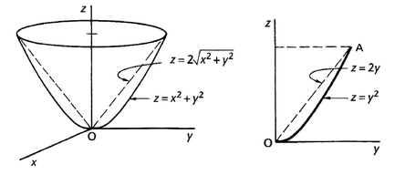
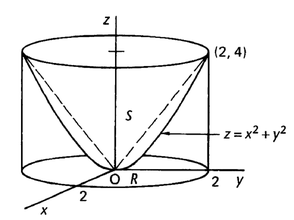
Find the area of the surface $S$ of the paraboloid $z = x^2+y^2$ cut off by the cone $z = 2\sqrt{x^2+y^2}$

Solution

We can find the point of intersection $A$ by considering the $y$-$z$ plane i.e. $x = 0$. Then, coordinates of $A$ are $A(2, 4)$.

The projection of the surface $S$ on the $x$-$y$ plane is

$x^2+y^2 = 4$

$A(S) = \iint_{R^*} \sqrt{1 + \left(\frac{\partial f}{\partial x}\right)^2 + \left(\frac{\partial f}{\partial y}\right)^2} dx\,dy$

For this we use the equation of the surface $S$. The information from the projection $R$ on the $x$-$y$ plane will later provide the limits of the two stages of integration.

For the time being, then

$A(S) = \iint_{R^*} \sqrt{1 + 4x^2 + 4y^2}\,dx\,dy$

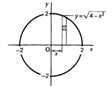
using Cartesian coordinates, we could integrate with respect to $y$ from $y = 0$ to $y = \sqrt{4-x^2}$ and then with respect to $x$ from $x = 0$ to $x = 2$. Finally we should multiply by four to cover all four quadrants

$\text{i.e. } A(S) = 4\int_{x=0}^{2}\int_{y=0}^{\sqrt{4-x^2}} \sqrt{1+4x^2+4y^2}\,dy\,dx$

but how do we carry out the actual integration? It becomes a lot easier if we use polar coordinates. The same integral in polar coordinates is

$A(S) = \int_{\theta=0}^{2\pi}\int_{r=0}^{2}\sqrt{1+4r^2}\,r\,dr\,d\theta$

$$\begin{aligned} A(S) &= \int_{\theta=0}^{2\pi}\int_{r=0}^{2}(1+4r^2)^{1/2}\,r\,dr\,d\theta = \int_0^{2\pi}\left[\frac{1}{12}(1+4r^2)^{3/2}\right]_0^2 d\theta \\ &= \frac{1}{12}\int_0^{2\pi}\{17^{3/2} - 1\}d\theta = 5.7577\,[\theta]_0^{2\pi} = 36.18 \end{aligned}$$

13.3 Some Properties of Surface Integral

In this section, we discuss some properties of surface integral that are relevant to solving the integral. In particular, we look into these two matters: (i) the orientation of a given surface, and (ii) the continuity of a surface.

13.3.1 Orientation of Surfaces

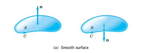
From (8) and (8*), we see that the value of the integral depends on the choice of the unit normal vector $\mathbf{n}$. We express this by saying that such an integral is an integral over an oriented surface $S$, that is, over a surface $S$ on which we have chosen one of the two possible unit normal vectors in a continuous fashion.

If we change the orientation of $S$, as illustrated by Figure 13.7, this means that we replace $\mathbf{n}$ with $-\mathbf{n}$. Then each component of $\mathbf{n}$ is multiplied by -1. This gives a negative to the original value of the surface integral.

Figure 13.7: Orientation of a Surface

Change of Orientation in a Surface Integral

The replacement of $\mathbf{n}$ by $-\mathbf{n}$ (hence of $\mathbf{N}$ by $-\mathbf{N}$) corresponds to the multiplication of the integral in (8) by -1

Example 13.7

From Example 13.1, for the surface $S$ represented by $\mathbf{r} = [u, u^2, v]$, $0 \leq u \leq 2$, $0 \leq v \leq 3$. If we consider the normal vector along the opposite direction:

Solution

$\mathbf{N} = \mathbf{r}_v \times \mathbf{r}_u = [0, 0, 1] \times [1, 2u, 0] = [-2u, 1, 0]$

$\mathbf{F}\cdot\mathbf{N} = [3v^2, 6, 6uv]\cdot[-2u, 1, 0] = 6 - 6uv^2$

Note that this integrand is now the negative of that in Example 13.1. Consequently, it is obvious that the integration also gives the negative of the value obtained in Example 13.1:

$\iint_S \mathbf{F}\cdot\mathbf{N}\,du\,dv = \int_0^3\int_0^2 (6 - 6uv^2)\,du\,dv = \int_0^3 (12 - 12v^2)\,dv = -72$

However, the orientation of a surface (the required direction of the unit normal vector) does not affect a scalar surface integral. This is because $\displaystyle\iint_S f(x,y,z)\,dS = \iint_S f(u,v)\left|\frac{\partial\mathbf{r}}{\partial u} \times \frac{\partial\mathbf{r}}{\partial v}\right| du\,dv$, so even though $\mathbf{r}_u \times \mathbf{r}_v = -(\mathbf{r}_v \times \mathbf{r}_u)$, the magnitudes are the same. In fact, we do not speak of orientation of the given surface when solving a scalar surface integral. Therefore, this is also sometimes known as surface integral without regard to orientation.

13.3.2 Continuity of Surfaces

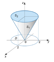
This property is similar to that of a line integral. Its concept can be conveniently expressed by: $\iint f(x,y,z)\,dS = \iint f(x,y,z)\,dS_1 + \iint f(x,y,z)\,dS_2$ for ease of understanding. This means, when the integration is to be carried out over a surface $S$ which is a composite of two (or more) surfaces, e.g. $S_1$ and $S_2$, the surface integral can be obtained by summing all the component surface integrals. This is true as long as the piecewise surface is continuous.

This property is usually applicable in situations involving closed surfaces, for example, as illustrated below:

Example 13.8

Evaluate the surface integral $\displaystyle\iint_S (z^2)\,dS$, where $S$ is the total area of the cone $\sqrt{x^2+y^2} \leq z \leq 2$

Solution

$S_1$: surface of the cone

$S_2$: base (cover) of the cone

$S_1 = \iint_{S_1} z^2\,dS_1 = \sqrt{2}\iint x^2+y^2\,dx\,dy$

Change to polar coordinate

$= \sqrt{2}\int_0^{2\pi}\int_0^2 r^2\,r\,dr\,d\theta = 8\sqrt{2}\,\pi$

$S_2$ – base of the cone at $z = 2$

$S_2 = \iint_{S_2} 2^2\,dS_2 = 4\iint_{S_2} dS_2 \qquad \iint dS_2 = \text{area of the base} = \pi r^2 = \pi(2^2) = 4\pi$

$= 4\iint_{S_2} dS_2 = 4(4\pi) = 16\pi$

Total Surface Integral $= S_1 + S_2 = 8\sqrt{2}\pi + 16\pi$

As a final remark, note that this property is applicable to both scalar surface integrals and vector surface integrals.