Lecture 14: Stokes' Theorem Download the original PDF →
14.1 Introduction
From previous topic, we have learnt that double integrals over a region in the plane can be transformed into line integrals over the boundary curve of the region and conversely. We shall now see that more generally, surface integrals over a surface S S S C C C C C C
Stokes' theorem is the "curl analogue" of the divergence theorem and relates the integral of curl of a vector field over an open surface S S S C C C
If F \mathbf{F} F S S S c c c
∫ S curl F ⋅ d S = ∮ c F ⋅ d r \int_S \operatorname{curl} \mathbf{F} \cdot d\mathbf{S} = \oint_c \mathbf{F} \cdot d\mathbf{r} ∫ S curl F ⋅ d S = ∮ c F ⋅ d r This means that we can express a surface integral in terms of a line integral round the boundary curve.
Example 14.1
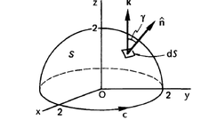
A hemisphere S S S x 2 + y 2 + z 2 = 4 x^2 + y^2 + z^2 = 4 x 2 + y 2 + z 2 = 4 z ≥ 0 z \geq 0 z ≥ 0 F = 2 y i − x j + x z k \mathbf{F} = 2y\mathbf{i} - x\mathbf{j} + xz\mathbf{k} F = 2 y i − x j + x z k c c c
Verify Stokes' theorem, that
∫ S curl F ⋅ d S = ∮ c F ⋅ d r \int_S \operatorname{curl} \mathbf{F} \cdot d\mathbf{S} = \oint_c \mathbf{F} \cdot d\mathbf{r} ∫ S curl F ⋅ d S = ∮ c F ⋅ d r
S : x 2 + y 2 + z 2 − 4 = 0 F = 2 y i − x j + x z k c is the circle x 2 + y 2 = 4 \begin{aligned}
S &: x^2 + y^2 + z^2 - 4 = 0 \\
\mathbf{F} &= 2y\mathbf{i} - x\mathbf{j} + xz\mathbf{k} \\
c &\text{ is the circle } x^2 + y^2 = 4
\end{aligned} S F c : x 2 + y 2 + z 2 − 4 = 0 = 2 y i − x j + x z k is the circle x 2 + y 2 = 4 (a)
∮ c F ⋅ d r = ∫ c ( 2 y i − x j + x z k ) ⋅ ( i d x + j d y + k d z ) = ∫ c ( 2 y d x − x d y + x z d z ) \begin{aligned}
\oint_c \mathbf{F} \cdot d\mathbf{r} &= \int_c (2y\mathbf{i} - x\mathbf{j} + xz\mathbf{k}) \cdot (\mathbf{i}\,dx + \mathbf{j}\,dy + \mathbf{k}\,dz) \\
&= \int_c (2y\,dx - x\,dy + xz\,dz)
\end{aligned} ∮ c F ⋅ d r = ∫ c ( 2 y i − x j + x z k ) ⋅ ( i d x + j d y + k d z ) = ∫ c ( 2 y d x − x d y + x z d z ) Converting to polar coordinates
x = 2 cos θ ; y = 2 sin θ ; z = 0 x = 2\cos\theta; \qquad y = 2\sin\theta; \qquad z = 0 x = 2 cos θ ; y = 2 sin θ ; z = 0
d x = − 2 sin θ d θ ; d y = 2 cos θ d θ ; limits θ = 0 to 2 π dx = -2\sin\theta\,d\theta; \qquad dy = 2\cos\theta\,d\theta; \qquad \text{limits } \theta = 0 \text{ to } 2\pi d x = − 2 sin θ d θ ; d y = 2 cos θ d θ ; limits θ = 0 to 2 π
Making the substitution and completing the integral
∮ c F ⋅ d r = ∫ 0 2 π ( 4 sin θ [ − 2 sin θ d θ ] − 2 cos θ 2 cos θ d θ ) \oint_c \mathbf{F} \cdot d\mathbf{r} = \int_0^{2\pi} \left(4\sin\theta[-2\sin\theta\,d\theta] - 2\cos\theta\,2\cos\theta\,d\theta\right) ∮ c F ⋅ d r = ∫ 0 2 π ( 4 sin θ [ − 2 sin θ d θ ] − 2 cos θ 2 cos θ d θ ) = − 4 ∫ 0 2 π ( 2 sin 2 θ + cos 2 θ ) d θ = − 4 ∫ 0 2 π ( 1 + sin 2 θ ) d θ = − 2 ∫ 0 2 π ( 3 − cos 2 θ ) d θ ( 1 ) = − 2 [ 3 θ − sin 2 θ 2 ] 0 2 π = − 12 π \begin{aligned}
&= -4\int_0^{2\pi} \left(2\sin^2\theta + \cos^2\theta\right) d\theta \\
&= -4\int_0^{2\pi} \left(1 + \sin^2\theta\right) d\theta = -2\int_0^{2\pi} \left(3 - \cos 2\theta\right) d\theta \qquad (1) \\
&= -2\left[3\theta - \frac{\sin 2\theta}{2}\right]_0^{2\pi} = -12\pi
\end{aligned} = − 4 ∫ 0 2 π ( 2 sin 2 θ + cos 2 θ ) d θ = − 4 ∫ 0 2 π ( 1 + sin 2 θ ) d θ = − 2 ∫ 0 2 π ( 3 − cos 2 θ ) d θ ( 1 ) = − 2 [ 3 θ − 2 sin 2 θ ] 0 2 π = − 12 π (b) Now we determine ∫ S curl F ⋅ d S \displaystyle \int_S \operatorname{curl} \mathbf{F} \cdot d\mathbf{S} ∫ S curl F ⋅ d S
∫ S curl F ⋅ d S = ∫ S curl F ⋅ n ^ d S \int_S \operatorname{curl} \mathbf{F} \cdot d\mathbf{S} = \int_S \operatorname{curl} \mathbf{F} \cdot \hat{\mathbf{n}} \; dS ∫ S curl F ⋅ d S = ∫ S curl F ⋅ n ^ d S curl F = ∣ i j k ∂ ∂ x ∂ ∂ y ∂ ∂ z 2 y − x x z ∣ = i ( 0 − 0 ) − j ( z − 0 ) + k ( − 1 − 2 ) = − z j − 3 k \operatorname{curl} \mathbf{F} = \begin{vmatrix} \mathbf{i} & \mathbf{j} & \mathbf{k} \\ \dfrac{\partial}{\partial x} & \dfrac{\partial}{\partial y} & \dfrac{\partial}{\partial z} \\ 2y & -x & xz \end{vmatrix} = \mathbf{i}(0-0) - \mathbf{j}(z-0) + \mathbf{k}(-1-2) = -z\mathbf{j} - 3\mathbf{k} curl F = i ∂ x ∂ 2 y j ∂ y ∂ − x k ∂ z ∂ x z = i ( 0 − 0 ) − j ( z − 0 ) + k ( − 1 − 2 ) = − z j − 3 k n = ∇ S ∣ ∇ S ∣ = 2 x i + 2 y j + 2 z k 4 x 2 + 4 y 2 + 4 z 2 = x i + y j + z k 2 \mathbf{n} = \frac{\nabla S}{|\nabla S|} = \frac{2x\mathbf{i} + 2y\mathbf{j} + 2z\mathbf{k}}{\sqrt{4x^2 + 4y^2 + 4z^2}} = \frac{x\mathbf{i} + y\mathbf{j} + z\mathbf{k}}{2} n = ∣∇ S ∣ ∇ S = 4 x 2 + 4 y 2 + 4 z 2 2 x i + 2 y j + 2 z k = 2 x i + y j + z k Now
Then ∫ S curl F ⋅ n ^ d S = ∫ S ( − z j − 3 k ) ⋅ ( x i + y j + z k 2 ) d S = 1 2 ∫ S ( − y z − 3 z ) d S \begin{aligned}
\text{Then } \int_S \operatorname{curl} \mathbf{F} \cdot \hat{\mathbf{n}} \; dS &= \int_S (-z\mathbf{j} - 3\mathbf{k}) \cdot \left(\frac{x\mathbf{i} + y\mathbf{j} + z\mathbf{k}}{2}\right) dS \\
&= \frac{1}{2}\int_S (-yz - 3z) \; dS
\end{aligned} Then ∫ S curl F ⋅ n ^ d S = ∫ S ( − z j − 3 k ) ⋅ ( 2 x i + y j + z k ) d S = 2 1 ∫ S ( − y z − 3 z ) d S Expressing this in spherical polar coordinates and integrating, because
x = 2 sin θ cos ϕ ; y = 2 sin θ sin ϕ ; z = 2 cos θ ; d S = 4 sin θ d θ d ϕ x = 2\sin\theta\cos\phi; \qquad y = 2\sin\theta\sin\phi; \qquad z = 2\cos\theta; \qquad dS = 4\sin\theta\,d\theta\,d\phi x = 2 sin θ cos ϕ ; y = 2 sin θ sin ϕ ; z = 2 cos θ ; d S = 4 sin θ d θ d ϕ
∴ ∫ S curl F ⋅ n ^ d S = 1 2 ∬ S ( − 2 sin θ sin ϕ 2 cos θ − 6 cos θ ) 4 sin θ d θ d ϕ = − 4 ∫ 0 2 π ∫ 0 π / 2 ( 2 sin 2 θ cos θ sin ϕ + 3 sin θ cos θ ) d θ d ϕ = − 4 ∫ 0 2 π [ 2 sin 3 θ sin ϕ 3 + 3 sin 2 θ 2 ] 0 π / 2 d ϕ ( 2 ) = − 4 ∫ 0 2 π ( 2 3 sin ϕ + 3 2 ) d ϕ = − 12 π \begin{aligned}
\therefore \int_S \operatorname{curl} \mathbf{F} \cdot \hat{\mathbf{n}} \; dS &= \frac{1}{2}\iint_S (-2\sin\theta\sin\phi\,2\cos\theta - 6\cos\theta)\,4\sin\theta\,d\theta\,d\phi \\
&= -4\int_0^{2\pi}\int_0^{\pi/2} \left(2\sin^2\theta\cos\theta\sin\phi + 3\sin\theta\cos\theta\right) d\theta\,d\phi \\
&= -4\int_0^{2\pi} \left[\frac{2\sin^3\theta\sin\phi}{3} + \frac{3\sin^2\theta}{2}\right]_0^{\pi/2} d\phi \qquad (2) \\
&= -4\int_0^{2\pi} \left(\frac{2}{3}\sin\phi + \frac{3}{2}\right) d\phi = -12\pi
\end{aligned} ∴ ∫ S curl F ⋅ n ^ d S = 2 1 ∬ S ( − 2 sin θ sin ϕ 2 cos θ − 6 cos θ ) 4 sin θ d θ d ϕ = − 4 ∫ 0 2 π ∫ 0 π /2 ( 2 sin 2 θ cos θ sin ϕ + 3 sin θ cos θ ) d θ d ϕ = − 4 ∫ 0 2 π [ 3 2 sin 3 θ sin ϕ + 2 3 sin 2 θ ] 0 π /2 d ϕ ( 2 ) = − 4 ∫ 0 2 π ( 3 2 sin ϕ + 2 3 ) d ϕ = − 12 π So we have from our two results (1) and (2)
∫ S curl F ⋅ d S = ∮ c F ⋅ d r \int_S \operatorname{curl} \mathbf{F} \cdot d\mathbf{S} = \oint_c \mathbf{F} \cdot d\mathbf{r} ∫ S curl F ⋅ d S = ∮ c F ⋅ d r Example 14.2
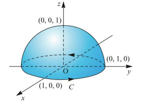
Verify the Stokes' Theorem for F = ( 2 x − y ) i − y z 2 j − y 2 z k \mathbf{F} = (2x-y)\mathbf{i} - yz^2\mathbf{j} - y^2z\mathbf{k} F = ( 2 x − y ) i − y z 2 j − y 2 z k S S S x 2 + y 2 + z 2 = 1 x^2 + y^2 + z^2 = 1 x 2 + y 2 + z 2 = 1 C C C
Hemispherical surface and boundary for Example 14.2
The surface and boundary involved are illustrated in the above figure. We are required to show that
∮ c F ⋅ d r = ∬ S curl F ⋅ d S \oint_c \mathbf{F} \cdot d\mathbf{r} = \iint_S \operatorname{curl} \mathbf{F} \cdot d\mathbf{S} ∮ c F ⋅ d r = ∬ S curl F ⋅ d S Since C C C ( x , y ) (x,y) ( x , y ) ∮ c F ⋅ d r \oint_c \mathbf{F} \cdot d\mathbf{r} ∮ c F ⋅ d r
x = cos ϕ , y = sin ϕ , x = \cos\phi, \qquad y = \sin\phi, x = cos ϕ , y = sin ϕ ,
so that
r = cos ϕ i + sin ϕ j \mathbf{r} = \cos\phi\,\mathbf{i} + \sin\phi\,\mathbf{j} r = cos ϕ i + sin ϕ j
giving
d r = − sin ϕ d ϕ i + cos ϕ d ϕ j d\mathbf{r} = -\sin\phi\,d\phi\,\mathbf{i} + \cos\phi\,d\phi\,\mathbf{j} d r = − sin ϕ d ϕ i + cos ϕ d ϕ j
Also, on the boundary C C C z = 0 z = 0 z = 0
F = ( 2 x − y ) i = ( 2 cos ϕ − sin ϕ ) i \mathbf{F} = (2x-y)\mathbf{i} = (2\cos\phi - \sin\phi)\mathbf{i} F = ( 2 x − y ) i = ( 2 cos ϕ − sin ϕ ) i
Thus,
∮ c F ⋅ d r = ∫ 0 2 π ( 2 cos ϕ − sin ϕ ) i ⋅ ( − sin ϕ i + cos ϕ j ) d ϕ = ∫ 0 2 π ( − 2 sin ϕ cos ϕ + sin 2 ϕ ) d ϕ = ∫ 0 2 π [ − sin 2 ϕ + 1 2 ( 1 − cos 2 ϕ ) ] d ϕ = π \begin{aligned}
\oint_c \mathbf{F} \cdot d\mathbf{r} &= \int_0^{2\pi} (2\cos\phi - \sin\phi)\mathbf{i} \cdot (-\sin\phi\,\mathbf{i} + \cos\phi\,\mathbf{j}) d\phi \\
&= \int_0^{2\pi} (-2\sin\phi\cos\phi + \sin^2\phi) d\phi = \int_0^{2\pi} \left[-\sin 2\phi + \frac{1}{2}(1 - \cos 2\phi)\right] d\phi = \pi
\end{aligned} ∮ c F ⋅ d r = ∫ 0 2 π ( 2 cos ϕ − sin ϕ ) i ⋅ ( − sin ϕ i + cos ϕ j ) d ϕ = ∫ 0 2 π ( − 2 sin ϕ cos ϕ + sin 2 ϕ ) d ϕ = ∫ 0 2 π [ − sin 2 ϕ + 2 1 ( 1 − cos 2 ϕ ) ] d ϕ = π curl F = ∣ i j k ∂ ∂ x ∂ ∂ y ∂ ∂ z 2 x − y − y z 2 − y 2 z ∣ = k \operatorname{curl} \mathbf{F} = \begin{vmatrix} \mathbf{i} & \mathbf{j} & \mathbf{k} \\ \dfrac{\partial}{\partial x} & \dfrac{\partial}{\partial y} & \dfrac{\partial}{\partial z} \\ 2x-y & -yz^2 & -y^2z \end{vmatrix} = \mathbf{k} curl F = i ∂ x ∂ 2 x − y j ∂ y ∂ − y z 2 k ∂ z ∂ − y 2 z = k The unit outward-drawn normal at a point ( x , y , z ) (x,y,z) ( x , y , z ) ( x i + y j + z k ) (x\mathbf{i} + y\mathbf{j} + z\mathbf{k}) ( x i + y j + z k ) x 2 + y 2 + z 2 = 1 x^2 + y^2 + z^2 = 1 x 2 + y 2 + z 2 = 1
∬ S curl F ⋅ d S = ∬ S k ⋅ ( x i + y j + z k ) d S = ∬ S z d S = ∫ 0 2 π ∫ 0 π / 2 cos θ sin θ d θ d ϕ = 2 π [ 1 2 sin 2 θ ] 0 π / 2 = π \begin{aligned}
\iint_S \operatorname{curl} \mathbf{F} \cdot d\mathbf{S} &= \iint_S \mathbf{k} \cdot (x\mathbf{i} + y\mathbf{j} + z\mathbf{k}) dS \\
&= \iint_S z \; dS = \int_0^{2\pi}\int_0^{\pi/2} \cos\theta\sin\theta \; d\theta\,d\phi = 2\pi\left[\frac{1}{2}\sin^2\theta\right]_0^{\pi/2} = \pi
\end{aligned} ∬ S curl F ⋅ d S = ∬ S k ⋅ ( x i + y j + z k ) d S = ∬ S z d S = ∫ 0 2 π ∫ 0 π /2 cos θ sin θ d θ d ϕ = 2 π [ 2 1 sin 2 θ ] 0 π /2 = π Hence ∮ c F ⋅ d r = ∬ S curl F ⋅ d S \oint_c \mathbf{F} \cdot d\mathbf{r} = \iint_S \operatorname{curl} \mathbf{F} \cdot d\mathbf{S} ∮ c F ⋅ d r = ∬ S curl F ⋅ d S
14.2 Direction of Unit Normal Vectors to a Surface
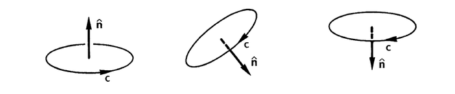
When we were dealing with the divergence theorem, the normal vectors were drawn in a direction outward from the enclosed region. With an open surface as we now have, there is in fact no inward or outward direction. With any general surface, a normal vector can be drawn in either of two opposite directions. To avoid confusion, a convention must therefore be agreed upon and the established rule is as follows.
A unit normal n ^ \hat{\mathbf{n}} n ^ S S S c c c
Example 14.3
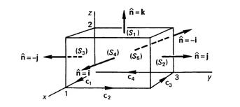
A surface consists of five sections formed by the planes x = 0 x=0 x = 0 x = 1 x=1 x = 1 y = 0 y=0 y = 0 y = 3 y=3 y = 3 z = 2 z=2 z = 2 F = y i + z 2 j + x y k \mathbf{F} = y\mathbf{i} + z^2\mathbf{j} + xy\mathbf{k} F = y i + z 2 j + x y k
If we progress round the boundary along c 1 c_1 c 1 c 2 c_2 c 2 c 3 c_3 c 3 c 4 c_4 c 4
We have to verify that
∫ S curl F ⋅ d S = ∮ c F ⋅ d r \int_S \operatorname{curl} \mathbf{F} \cdot d\mathbf{S} = \oint_c \mathbf{F} \cdot d\mathbf{r} ∫ S curl F ⋅ d S = ∮ c F ⋅ d r (a) We will start off by finding ∮ c F ⋅ d r \displaystyle \oint_c \mathbf{F} \cdot d\mathbf{r} ∮ c F ⋅ d r
(1) Along c 1 c_1 c 1 y = 0 y=0 y = 0 z = 0 z=0 z = 0 d y = 0 dy=0 d y = 0 d z = 0 dz=0 d z = 0
∴ ∫ c 1 F ⋅ d r = ∫ ( 0 + 0 + 0 ) = 0 \therefore \int_{c_1} \mathbf{F} \cdot d\mathbf{r} = \int (0 + 0 + 0) = 0 ∴ ∫ c 1 F ⋅ d r = ∫ ( 0 + 0 + 0 ) = 0
(2) Along c 2 c_2 c 2 x = 1 x=1 x = 1 z = 0 z=0 z = 0 d x = 0 dx=0 d x = 0 d z = 0 dz=0 d z = 0
∴ ∫ c 2 F ⋅ d r = ∫ ( 0 + 0 + 0 ) = 0 \therefore \int_{c_2} \mathbf{F} \cdot d\mathbf{r} = \int (0 + 0 + 0) = 0 ∴ ∫ c 2 F ⋅ d r = ∫ ( 0 + 0 + 0 ) = 0
(3) Along c 3 c_3 c 3 y = 3 y=3 y = 3 z = 0 z=0 z = 0 d y = 0 dy=0 d y = 0 d z = 0 dz=0 d z = 0
∴ ∫ c 3 F ⋅ d r = ∫ 1 0 ( 3 d x + 0 + 0 ) = [ 3 x ] 1 0 = − 3 \therefore \int_{c_3} \mathbf{F} \cdot d\mathbf{r} = \int_1^0 (3\,dx + 0 + 0) = [3x]_1^0 = -3 ∴ ∫ c 3 F ⋅ d r = ∫ 1 0 ( 3 d x + 0 + 0 ) = [ 3 x ] 1 0 = − 3
(4) Along c 4 c_4 c 4 x = 0 x=0 x = 0 z = 0 z=0 z = 0 d x = 0 dx=0 d x = 0 d z = 0 dz=0 d z = 0
∴ ∫ c 4 F ⋅ d r = ∫ ( 0 + 0 + 0 ) = 0 \therefore \int_{c_4} \mathbf{F} \cdot d\mathbf{r} = \int (0 + 0 + 0) = 0 ∴ ∫ c 4 F ⋅ d r = ∫ ( 0 + 0 + 0 ) = 0
∴ ∮ c F ⋅ d r = 0 + 0 − 3 + 0 = − 3 \therefore \oint_c \mathbf{F} \cdot d\mathbf{r} = 0 + 0 - 3 + 0 = -3 ∴ ∮ c F ⋅ d r = 0 + 0 − 3 + 0 = − 3
∮ c F ⋅ d r = − 3 \oint_c \mathbf{F} \cdot d\mathbf{r} = -3 ∮ c F ⋅ d r = − 3
(b) Now we have to find ∫ S curl F ⋅ d S \displaystyle \int_S \operatorname{curl} \mathbf{F} \cdot d\mathbf{S} ∫ S curl F ⋅ d S
First we need an expression for curl F \mathbf{F} F
F = y i + z 2 j + x y k \mathbf{F} = y\mathbf{i} + z^2\mathbf{j} + xy\mathbf{k} F = y i + z 2 j + x y k
curl F = ∇ × F = ∣ i j k ∂ ∂ x ∂ ∂ y ∂ ∂ z y z 2 x y ∣ = i ( x − 2 z ) − j ( y − 0 ) + k ( 0 − 1 ) = ( x − 2 z ) i − y j − k \operatorname{curl} \mathbf{F} = \nabla \times \mathbf{F} = \begin{vmatrix} \mathbf{i} & \mathbf{j} & \mathbf{k} \\ \dfrac{\partial}{\partial x} & \dfrac{\partial}{\partial y} & \dfrac{\partial}{\partial z} \\ y & z^2 & xy \end{vmatrix} = \mathbf{i}(x-2z) - \mathbf{j}(y-0) + \mathbf{k}(0-1) = (x-2z)\mathbf{i} - y\mathbf{j} - \mathbf{k} curl F = ∇ × F = i ∂ x ∂ y j ∂ y ∂ z 2 k ∂ z ∂ x y = i ( x − 2 z ) − j ( y − 0 ) + k ( 0 − 1 ) = ( x − 2 z ) i − y j − k Then for each section, we obtain ∫ S curl F ⋅ d S = ∫ S curl F ⋅ n ^ d S \displaystyle \int_S \operatorname{curl} \mathbf{F} \cdot d\mathbf{S} = \int_S \operatorname{curl} \mathbf{F} \cdot \hat{\mathbf{n}} \; dS ∫ S curl F ⋅ d S = ∫ S curl F ⋅ n ^ d S
(1) S 1 S_1 S 1 n ^ = k \hat{\mathbf{n}} = \mathbf{k} n ^ = k
∫ S 1 curl F ⋅ n ^ d S = ∫ S 1 [ ( x − 2 z ) i − y j − k ] ⋅ ( k ) d S \int_{S_1} \operatorname{curl} \mathbf{F} \cdot \hat{\mathbf{n}} \; dS = \int_{S_1} [(x-2z)\mathbf{i} - y\mathbf{j} - \mathbf{k}] \cdot (\mathbf{k}) \; dS ∫ S 1 curl F ⋅ n ^ d S = ∫ S 1 [( x − 2 z ) i − y j − k ] ⋅ ( k ) d S ∫ S 1 ( − 1 ) d S = − ( area of S 1 ) = − 3 \int_{S_1} (-1) \, dS = -(\text{area of } S_1) = -3 ∫ S 1 ( − 1 ) d S = − ( area of S 1 ) = − 3 Then, likewise
(2) S 2 S_2 S 2 n ^ = j \hat{\mathbf{n}} = \mathbf{j} n ^ = j
∴ ∫ S 2 curl F ⋅ n ^ d S = ∫ S 2 [ ( x − 2 z ) i − y j − k ] ⋅ ( j ) d S = ∫ S 2 ( − y ) d S \begin{aligned}
\therefore \int_{S_2} \operatorname{curl} \mathbf{F} \cdot \hat{\mathbf{n}} \; dS &= \int_{S_2} [(x-2z)\mathbf{i} - y\mathbf{j} - \mathbf{k}] \cdot (\mathbf{j}) \; dS \\
&= \int_{S_2} (-y) \; dS
\end{aligned} ∴ ∫ S 2 curl F ⋅ n ^ d S = ∫ S 2 [( x − 2 z ) i − y j − k ] ⋅ ( j ) d S = ∫ S 2 ( − y ) d S But y = 3 y=3 y = 3
∴ ∫ S 2 curl F ⋅ n ^ d S = ∫ S 2 ( − 3 ) d S = ( − 3 ) ( 2 ) = − 6 \therefore \int_{S_2} \operatorname{curl} \mathbf{F} \cdot \hat{\mathbf{n}} \; dS = \int_{S_2} (-3) \, dS = (-3)(2) = -6 ∴ ∫ S 2 curl F ⋅ n ^ d S = ∫ S 2 ( − 3 ) d S = ( − 3 ) ( 2 ) = − 6
(3) S 3 S_3 S 3 n ^ = − j \hat{\mathbf{n}} = -\mathbf{j} n ^ = − j
∫ S 3 curl F ⋅ n ^ d S = ∫ S 3 [ ( x − 2 z ) i − y j − k ] ⋅ ( − j ) d S = ∫ S 3 ( y ) d S \begin{aligned}
\int_{S_3} \operatorname{curl} \mathbf{F} \cdot \hat{\mathbf{n}} \; dS &= \int_{S_3} [(x-2z)\mathbf{i} - y\mathbf{j} - \mathbf{k}] \cdot (-\mathbf{j}) \; dS \\
&= \int_{S_3} (y) \; dS
\end{aligned} ∫ S 3 curl F ⋅ n ^ d S = ∫ S 3 [( x − 2 z ) i − y j − k ] ⋅ ( − j ) d S = ∫ S 3 ( y ) d S But y = 0 y=0 y = 0 S 3 S_3 S 3
∴ ∫ S 3 curl F ⋅ n ^ d S = 0 \therefore \int_{S_3} \operatorname{curl} \mathbf{F} \cdot \hat{\mathbf{n}} \; dS = 0 ∴ ∫ S 3 curl F ⋅ n ^ d S = 0
(4) S 4 S_4 S 4 n ^ = i \hat{\mathbf{n}} = \mathbf{i} n ^ = i
∴ ∫ S 4 curl F ⋅ n ^ d S = ∫ S 4 [ ( x − 2 z ) i − y j − k ] ⋅ ( i ) d S = ∫ S 4 ( x − 2 z ) d S \begin{aligned}
\therefore \int_{S_4} \operatorname{curl} \mathbf{F} \cdot \hat{\mathbf{n}} \; dS &= \int_{S_4} [(x-2z)\mathbf{i} - y\mathbf{j} - \mathbf{k}] \cdot (\mathbf{i}) \; dS \\
&= \int_{S_4} (x-2z) \; dS
\end{aligned} ∴ ∫ S 4 curl F ⋅ n ^ d S = ∫ S 4 [( x − 2 z ) i − y j − k ] ⋅ ( i ) d S = ∫ S 4 ( x − 2 z ) d S but x = 1 x=1 x = 1 S 4 S_4 S 4
∴ ∫ S 4 curl F ⋅ n ^ d S = ∫ 0 3 ∫ 0 2 ( 1 − 2 z ) d z d y = ∫ 0 3 [ z − z 2 ] 0 2 d y = ∫ 0 3 ( − 2 ) d y = [ − 2 y ] 0 3 = − 6 \begin{aligned}
\therefore \int_{S_4} \operatorname{curl} \mathbf{F} \cdot \hat{\mathbf{n}} \; dS &= \int_0^3\int_0^2 (1-2z)\,dz\,dy = \int_0^3 \left[z - z^2\right]_0^2 dy \\
&= \int_0^3 (-2) \; dy = [-2y]_0^3 = -6
\end{aligned} ∴ ∫ S 4 curl F ⋅ n ^ d S = ∫ 0 3 ∫ 0 2 ( 1 − 2 z ) d z d y = ∫ 0 3 [ z − z 2 ] 0 2 d y = ∫ 0 3 ( − 2 ) d y = [ − 2 y ] 0 3 = − 6 (5) S 5 S_5 S 5 n ^ = − i \hat{\mathbf{n}} = -\mathbf{i} n ^ = − i x = 0 x=0 x = 0 S 5 S_5 S 5
Similar working to the above gives ∫ S 5 curl F ⋅ n ^ d S = 12 \displaystyle \int_{S_5} \operatorname{curl} \mathbf{F} \cdot \hat{\mathbf{n}} \; dS = 12 ∫ S 5 curl F ⋅ n ^ d S = 12
Finally, collecting the five results together gives
∴ ∫ S curl F ⋅ n ^ d S = − 3 − 6 + 0 − 6 + 12 = − 3 \therefore \int_S \operatorname{curl} \mathbf{F} \cdot \hat{\mathbf{n}} \; dS = -3 - 6 + 0 - 6 + 12 = -3 ∴ ∫ S curl F ⋅ n ^ d S = − 3 − 6 + 0 − 6 + 12 = − 3
So, referring back to our result for section (a) we see that
∫ S curl F ⋅ d S = ∮ c F ⋅ d r \int_S \operatorname{curl} \mathbf{F} \cdot d\mathbf{S} = \oint_c \mathbf{F} \cdot d\mathbf{r} ∫ S curl F ⋅ d S = ∮ c F ⋅ d r Example 14.4
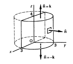
A surface S S S x 2 + y 2 = 9 x^2 + y^2 = 9 x 2 + y 2 = 9 z = 0 z=0 z = 0 z = 4 z=4 z = 4 y ≥ 0 y \geq 0 y ≥ 0 z = 0 z=0 z = 0 z = 4 z=4 z = 4 F = z i + x y j + x z k \mathbf{F} = z\mathbf{i} + xy\mathbf{j} + xz\mathbf{k} F = z i + x y j + x z k ∫ S curl F ⋅ d S \displaystyle \int_S \operatorname{curl} \mathbf{F} \cdot d\mathbf{S} ∫ S curl F ⋅ d S
The surface S S S
(a) The curved surface of the cylinder
(b) The top and bottom semicircles
We could therefore evaluate
∫ S curl F ⋅ d S \int_S \operatorname{curl} \mathbf{F} \cdot d\mathbf{S} ∫ S curl F ⋅ d S
Over each of these separately.
However, we know by Stokes' theorem that
F = z i + x y j + x z k \mathbf{F} = z\mathbf{i} + xy\mathbf{j} + xz\mathbf{k} F = z i + x y j + x z k
∮ c F ⋅ d r = ∮ c ( z i + x y j + x z k ) ⋅ ( i d x + j d y + k d z ) = ∮ c ( z d x + x y d y + x z d z ) \begin{aligned}
\oint_c \mathbf{F} \cdot d\mathbf{r} &= \oint_c (z\mathbf{i} + xy\mathbf{j} + xz\mathbf{k}) \cdot (\mathbf{i}\,dx + \mathbf{j}\,dy + \mathbf{k}\,dz) \\
&= \oint_c (z\,dx + xy\,dy + xz\,dz)
\end{aligned} ∮ c F ⋅ d r = ∮ c ( z i + x y j + x z k ) ⋅ ( i d x + j d y + k d z ) = ∮ c ( z d x + x y d y + x z d z ) Now we can work through this easily enough, taking c 1 c_1 c 1 c 2 c_2 c 2 c 3 c_3 c 3 c 4 c_4 c 4
∫ S curl F ⋅ d S = ∮ c F ⋅ d r = ∮ c ( z d x + x y d y + x z d z ) \int_S \operatorname{curl} \mathbf{F} \cdot d\mathbf{S} = \oint_c \mathbf{F} \cdot d\mathbf{r} = \oint_c (z\,dx + xy\,dy + xz\,dz) ∫ S curl F ⋅ d S = ∮ c F ⋅ d r = ∮ c ( z d x + x y d y + x z d z ) (1) C 1 C_1 C 1 y = 0 y=0 y = 0 z = 0 z=0 z = 0 d y = 0 dy=0 d y = 0 d z = 0 dz=0 d z = 0
∫ c 1 F ⋅ d r = ∫ c 1 ( 0 + 0 + 0 ) = 0 \int_{c_1} \mathbf{F} \cdot d\mathbf{r} = \int_{c_1} (0 + 0 + 0) = 0 ∫ c 1 F ⋅ d r = ∫ c 1 ( 0 + 0 + 0 ) = 0
(2) C 2 C_2 C 2 x = − 3 x=-3 x = − 3 y = 0 y=0 y = 0 d x = 0 dx=0 d x = 0 d y = 0 dy=0 d y = 0
∫ c 2 F ⋅ d r = ∫ c 2 ( 0 + 0 − 3 z d z ) = [ − 3 z 2 2 ] 0 4 = − 24 \int_{c_2} \mathbf{F} \cdot d\mathbf{r} = \int_{c_2} (0 + 0 - 3z\,dz) = \left[\frac{-3z^2}{2}\right]_0^4 = -24 ∫ c 2 F ⋅ d r = ∫ c 2 ( 0 + 0 − 3 z d z ) = [ 2 − 3 z 2 ] 0 4 = − 24
(3) C 3 C_3 C 3 y = 0 y=0 y = 0 z = 4 z=4 z = 4 d y = 0 dy=0 d y = 0 d z = 0 dz=0 d z = 0
∫ c 3 F ⋅ d r = ∫ c 3 ( 4 d x + 0 + 0 ) = ∫ − 3 3 4 d x = 24 \int_{c_3} \mathbf{F} \cdot d\mathbf{r} = \int_{c_3} (4\,dx + 0 + 0) = \int_{-3}^{3} 4\,dx = 24 ∫ c 3 F ⋅ d r = ∫ c 3 ( 4 d x + 0 + 0 ) = ∫ − 3 3 4 d x = 24
(4) C 4 C_4 C 4 x = 3 x=3 x = 3 y = 0 y=0 y = 0 d x = 0 dx=0 d x = 0 d y = 0 dy=0 d y = 0
∫ c 4 F ⋅ d r = ∫ c 4 ( 0 + 0 + 3 z d z ) = [ 3 z 2 2 ] 4 0 = − 24 \int_{c_4} \mathbf{F} \cdot d\mathbf{r} = \int_{c_4} (0 + 0 + 3z\,dz) = \left[\frac{3z^2}{2}\right]_4^0 = -24 ∫ c 4 F ⋅ d r = ∫ c 4 ( 0 + 0 + 3 z d z ) = [ 2 3 z 2 ] 4 0 = − 24
There is an alternative way of solving this example. We can consider a fictitious surface enclosed by the rectangular curve C 1 C_1 C 1 C 2 C_2 C 2 C 3 C_3 C 3 C 4 C_4 C 4 ∫ S curl F ⋅ d S \displaystyle \int_S \operatorname{curl} \mathbf{F} \cdot d\mathbf{S} ∫ S curl F ⋅ d S y = 0 y = 0 y = 0 − 3 ≤ x ≤ 3 -3 \leq x \leq 3 − 3 ≤ x ≤ 3 0 ≤ z ≤ 4 0 \leq z \leq 4 0 ≤ z ≤ 4
curl F = ∣ i j k ∂ ∂ x ∂ ∂ y ∂ ∂ z z x y x z ∣ = ( 1 − z ) j + y k \operatorname{curl} \mathbf{F} = \begin{vmatrix} \mathbf{i} & \mathbf{j} & \mathbf{k} \\ \dfrac{\partial}{\partial x} & \dfrac{\partial}{\partial y} & \dfrac{\partial}{\partial z} \\ z & xy & xz \end{vmatrix} = (1-z)\mathbf{j} + y\mathbf{k} curl F = i ∂ x ∂ z j ∂ y ∂ x y k ∂ z ∂ x z = ( 1 − z ) j + y k For this vertical rectangular surface, unit normal vector, n ^ = j \hat{\mathbf{n}} = \mathbf{j} n ^ = j
∫ S curl F ⋅ d S = ∫ S curl F ⋅ n ^ d S = ∫ − 3 3 ∫ 0 4 ( 1 − z ) d z d x = ∫ − 3 3 [ z − z 2 2 ] 0 4 d x = ∫ − 3 3 − 4 d x = − 24 \begin{aligned}
\int_S \operatorname{curl} \mathbf{F} \cdot d\mathbf{S} &= \int_S \operatorname{curl} \mathbf{F} \cdot \hat{\mathbf{n}} \; dS \\
&= \int_{-3}^3\int_0^4 (1-z)\,dz\,dx \\
&= \int_{-3}^3 \left[z - \frac{z^2}{2}\right]_0^4 dx \\
&= \int_{-3}^3 -4 \; dx = -24
\end{aligned} ∫ S curl F ⋅ d S = ∫ S curl F ⋅ n ^ d S = ∫ − 3 3 ∫ 0 4 ( 1 − z ) d z d x = ∫ − 3 3 [ z − 2 z 2 ] 0 4 d x = ∫ − 3 3 − 4 d x = − 24 This alternative solution demonstrates an interesting property related to Stokes' theorem: if two or more surfaces share the same closed curve, their surface integrals (of the Stokes' theorem) give the same value.
Green's theorem enables an integral over a plane area to be expressed in terms of a line integral round its boundary curve. Let P P P Q Q Q x x x y y y c c c R R R x x x y y y
If the first partial derivatives are continuous within the region and on the boundary, then Green's theorem states that
∬ R ( ∂ P ∂ y − ∂ Q ∂ x ) d x d y = − ∮ c ( P d x + Q d y ) \iint_R \left(\frac{\partial P}{\partial y} - \frac{\partial Q}{\partial x}\right) dx\,dy = -\oint_c (P\,dx + Q\,dy) ∬ R ( ∂ y ∂ P − ∂ x ∂ Q ) d x d y = − ∮ c ( P d x + Q d y ) That is, a double integral over the plane region R R R c c c
If P P P Q Q Q x x x y y y S S S c c c
∮ c ( P d x + Q d y ) = ∬ S ( ∂ Q ∂ x − ∂ P ∂ y ) d x d y \oint_c (P\,dx + Q\,dy) = \iint_S \left(\frac{\partial Q}{\partial x} - \frac{\partial P}{\partial y}\right) dx\,dy ∮ c ( P d x + Q d y ) = ∬ S ( ∂ x ∂ Q − ∂ y ∂ P ) d x d y where the line integral is taken round c c c
S S S c c c
RHS: d S = d x d y dS = dx\,dy d S = d x d y
d S = n ^ d S = k d x d y d\mathbf{S} = \hat{\mathbf{n}} \; dS = \mathbf{k} \; dx\,dy d S = n ^ d S = k d x d y
If F = P i + Q j \mathbf{F} = P\mathbf{i} + Q\mathbf{j} F = P i + Q j P = P ( x , y ) P = P(x,y) P = P ( x , y ) Q = Q ( x , y ) Q = Q(x,y) Q = Q ( x , y )
curl F = ∣ i j k ∂ ∂ x ∂ ∂ y ∂ ∂ z P Q 0 ∣ = i ( 0 − ∂ Q ∂ z ) − j ( 0 − ∂ P ∂ z ) + k ( ∂ Q ∂ x − ∂ P ∂ y ) \operatorname{curl} \mathbf{F} = \begin{vmatrix} \mathbf{i} & \mathbf{j} & \mathbf{k} \\ \dfrac{\partial}{\partial x} & \dfrac{\partial}{\partial y} & \dfrac{\partial}{\partial z} \\ P & Q & 0 \end{vmatrix} = \mathbf{i}\left(0 - \frac{\partial Q}{\partial z}\right) - \mathbf{j}\left(0 - \frac{\partial P}{\partial z}\right) + \mathbf{k}\left(\frac{\partial Q}{\partial x} - \frac{\partial P}{\partial y}\right) curl F = i ∂ x ∂ P j ∂ y ∂ Q k ∂ z ∂ 0 = i ( 0 − ∂ z ∂ Q ) − j ( 0 − ∂ z ∂ P ) + k ( ∂ x ∂ Q − ∂ y ∂ P ) But in the x x x y y y ∂ Q ∂ z = ∂ P ∂ z = 0 \dfrac{\partial Q}{\partial z} = \dfrac{\partial P}{\partial z} = 0 ∂ z ∂ Q = ∂ z ∂ P = 0 ∴ curl F = k ( ∂ Q ∂ x − ∂ P ∂ y ) \therefore \operatorname{curl} \mathbf{F} = \mathbf{k}\left(\dfrac{\partial Q}{\partial x} - \dfrac{\partial P}{\partial y}\right) ∴ curl F = k ( ∂ x ∂ Q − ∂ y ∂ P )
So ∫ S curl F ⋅ d S = ∫ S curl F ⋅ n ^ d S \displaystyle \int_S \operatorname{curl} \mathbf{F} \cdot d\mathbf{S} = \int_S \operatorname{curl} \mathbf{F} \cdot \hat{\mathbf{n}} \; dS ∫ S curl F ⋅ d S = ∫ S curl F ⋅ n ^ d S x x x y y y n ^ = k \hat{\mathbf{n}} = \mathbf{k} n ^ = k
∴ ∫ S curl F ⋅ d S = ∫ S k ( ∂ Q ∂ x − ∂ P ∂ y ) ⋅ ( k ) d S = ∬ S ( ∂ Q ∂ x − ∂ P ∂ y ) d x d y \therefore \int_S \operatorname{curl} \mathbf{F} \cdot d\mathbf{S} = \int_S \mathbf{k}\left(\frac{\partial Q}{\partial x} - \frac{\partial P}{\partial y}\right) \cdot (\mathbf{k}) \, dS = \iint_S \left(\frac{\partial Q}{\partial x} - \frac{\partial P}{\partial y}\right) dx\,dy ∴ ∫ S curl F ⋅ d S = ∫ S k ( ∂ x ∂ Q − ∂ y ∂ P ) ⋅ ( k ) d S = ∬ S ( ∂ x ∂ Q − ∂ y ∂ P ) d x d y ∴ ∫ S curl F ⋅ d S = ∬ S ( ∂ Q ∂ x − ∂ P ∂ y ) d x d y ( 1 ) \therefore \int_S \operatorname{curl} \mathbf{F} \cdot d\mathbf{S} = \iint_S \left(\frac{\partial Q}{\partial x} - \frac{\partial P}{\partial y}\right) dx\,dy \qquad (1) ∴ ∫ S curl F ⋅ d S = ∬ S ( ∂ x ∂ Q − ∂ y ∂ P ) d x d y ( 1 ) Now by Stokes' theorem
∫ S curl F ⋅ d S = ∮ c F ⋅ d r \int_S \operatorname{curl} \mathbf{F} \cdot d\mathbf{S} = \oint_c \mathbf{F} \cdot d\mathbf{r} ∫ S curl F ⋅ d S = ∮ c F ⋅ d r
LHS: in this case
∮ c F ⋅ d r = ∮ c ( P i + Q j ) ⋅ ( i d x + j d y + k d z ) = ∮ c ( P d x + Q d y ) \begin{aligned}
\oint_c \mathbf{F} \cdot d\mathbf{r} &= \oint_c (P\mathbf{i} + Q\mathbf{j}) \cdot (\mathbf{i}\,dx + \mathbf{j}\,dy + \mathbf{k}\,dz) \\
&= \oint_c (P\,dx + Q\,dy)
\end{aligned} ∮ c F ⋅ d r = ∮ c ( P i + Q j ) ⋅ ( i d x + j d y + k d z ) = ∮ c ( P d x + Q d y ) ∴ ∮ c F ⋅ d r = ∮ c P d x + Q d y ( 2 ) \therefore \oint_c \mathbf{F} \cdot d\mathbf{r} = \oint_c P\,dx + Q\,dy \qquad (2) ∴ ∮ c F ⋅ d r = ∮ c P d x + Q d y ( 2 )
Therefore from (1) and (2)
Stokes' theorem ∫ S curl F ⋅ d S = ∮ c F ⋅ d r \displaystyle \int_S \operatorname{curl} \mathbf{F} \cdot d\mathbf{S} = \oint_c \mathbf{F} \cdot d\mathbf{r} ∫ S curl F ⋅ d S = ∮ c F ⋅ d r
∬ S ( ∂ Q ∂ x − ∂ P ∂ y ) d x d y = ∮ c P d x + Q d y \iint_S \left(\frac{\partial Q}{\partial x} - \frac{\partial P}{\partial y}\right) dx\,dy = \oint_c P\,dx + Q\,dy ∬ S ( ∂ x ∂ Q − ∂ y ∂ P ) d x d y = ∮ c P d x + Q d y Example 14.5
Verify Green's theorem for the integral ∮ c [ ( x 2 + y 2 ) d x + ( x + 2 y ) d y ] \displaystyle \oint_c \left[(x^2 + y^2)dx + (x + 2y)dy\right] ∮ c [ ( x 2 + y 2 ) d x + ( x + 2 y ) d y ] c c c
y = 0 0 ≤ x ≤ 2 x 2 + y 2 = 4 0 ≤ x ≤ 2 x = 0 0 ≤ y ≤ 2 \begin{aligned}
y &= 0 & 0 &\leq x \leq 2 \\
x^2 + y^2 &= 4 & 0 &\leq x \leq 2 \\
x &= 0 & 0 &\leq y \leq 2
\end{aligned} y x 2 + y 2 x = 0 = 4 = 0 0 0 0 ≤ x ≤ 2 ≤ x ≤ 2 ≤ y ≤ 2
Green's theorem: ∬ S ( ∂ Q ∂ x − ∂ P ∂ y ) d x d y = ∮ c ( P d x + Q d y ) \displaystyle \iint_S \left(\frac{\partial Q}{\partial x} - \frac{\partial P}{\partial y}\right) dx\,dy = \oint_c (P\,dx + Q\,dy) ∬ S ( ∂ x ∂ Q − ∂ y ∂ P ) d x d y = ∮ c ( P d x + Q d y )
In this case ( x 2 + y 2 ) d x + ( x + 2 y ) d y = P d x + Q d y (x^2 + y^2)dx + (x + 2y)dy = P\,dx + Q\,dy ( x 2 + y 2 ) d x + ( x + 2 y ) d y = P d x + Q d y
∴ P = x 2 + y 2 and Q = x + 2 y \therefore P = x^2 + y^2 \quad \text{and} \quad Q = x + 2y ∴ P = x 2 + y 2 and Q = x + 2 y
We now take c 1 c_1 c 1 c 2 c_2 c 2 c 3 c_3 c 3
(1) c 1 c_1 c 1 y = 0 y=0 y = 0 d y = 0 dy=0 d y = 0
∴ ∫ c 1 ( P d x + Q d y ) = ∫ 0 2 x 2 d x = [ x 3 3 ] 0 2 = 8 3 \therefore \int_{c_1} (P\,dx + Q\,dy) = \int_0^2 x^2\,dx = \left[\frac{x^3}{3}\right]_0^2 = \frac{8}{3} ∴ ∫ c 1 ( P d x + Q d y ) = ∫ 0 2 x 2 d x = [ 3 x 3 ] 0 2 = 3 8
(2) c 2 c_2 c 2
x 2 + y 2 = 4 ∴ y 2 = 4 − x 2 ∴ y = ( 4 − x 2 ) 1 / 2 x + 2 y = x + 2 ( 4 − x 2 ) 1 / 2 d y = 1 2 ( 4 − x 2 ) − 1 / 2 ( − 2 x ) d x = − x 4 − x 2 d x \begin{aligned}
x^2 + y^2 &= 4 \quad \therefore y^2 = 4 - x^2 \quad \therefore y = (4 - x^2)^{1/2} \\
x + 2y &= x + 2(4 - x^2)^{1/2} \\
dy &= \frac{1}{2}(4 - x^2)^{-1/2}(-2x)dx = \frac{-x}{\sqrt{4 - x^2}} \, dx
\end{aligned} x 2 + y 2 x + 2 y d y = 4 ∴ y 2 = 4 − x 2 ∴ y = ( 4 − x 2 ) 1/2 = x + 2 ( 4 − x 2 ) 1/2 = 2 1 ( 4 − x 2 ) − 1/2 ( − 2 x ) d x = 4 − x 2 − x d x ∴ ∫ c 2 ( P d x + Q d y ) = ∫ c 2 [ 4 + ( x + 2 4 − x 2 ) ( − x 4 − x 2 ) ] d x = ∫ c 2 [ 4 − 2 x − x 2 4 − x 2 ] d x \begin{aligned}
\therefore \int_{c_2} (P\,dx + Q\,dy) &= \int_{c_2} \left[4 + \left(x + 2\sqrt{4-x^2}\right)\left(\frac{-x}{\sqrt{4-x^2}}\right)\right] dx \\
&= \int_{c_2} \left[4 - 2x - \frac{x^2}{\sqrt{4-x^2}}\right] dx
\end{aligned} ∴ ∫ c 2 ( P d x + Q d y ) = ∫ c 2 [ 4 + ( x + 2 4 − x 2 ) ( 4 − x 2 − x ) ] d x = ∫ c 2 [ 4 − 2 x − 4 − x 2 x 2 ] d x Putting x = 2 sin θ x = 2\sin\theta x = 2 sin θ 4 − x 2 = 2 cos θ \sqrt{4-x^2} = 2\cos\theta 4 − x 2 = 2 cos θ d x = 2 cos θ d θ dx = 2\cos\theta\,d\theta d x = 2 cos θ d θ
Limits: x = 2 x=2 x = 2 θ = π 2 \theta = \dfrac{\pi}{2} θ = 2 π x = 0 \qquad x=0 x = 0 θ = 0 \theta = 0 θ = 0
∴ ∫ c 2 ( P d x + Q d y ) = ∫ π / 2 0 [ 4 − 4 sin θ − 4 sin 2 θ 2 cos θ ] 2 cos θ d θ = 4 [ 2 sin θ − sin 2 θ − 1 2 ( θ − sin 2 θ 2 ) ] π / 2 0 = 4 [ − ( 2 − 1 − π 4 ) ] = π − 4 \begin{aligned}
\therefore \int_{c_2} (P\,dx + Q\,dy) &= \int_{\pi/2}^{0} \left[4 - 4\sin\theta - \frac{4\sin^2\theta}{2\cos\theta}\right] 2\cos\theta \, d\theta \\
&= 4\left[2\sin\theta - \sin^2\theta - \frac{1}{2}\left(\theta - \frac{\sin 2\theta}{2}\right)\right]_{\pi/2}^{0} \\
&= 4\left[-\left(2 - 1 - \frac{\pi}{4}\right)\right] = \pi - 4
\end{aligned} ∴ ∫ c 2 ( P d x + Q d y ) = ∫ π /2 0 [ 4 − 4 sin θ − 2 cos θ 4 sin 2 θ ] 2 cos θ d θ = 4 [ 2 sin θ − sin 2 θ − 2 1 ( θ − 2 sin 2 θ ) ] π /2 0 = 4 [ − ( 2 − 1 − 4 π ) ] = π − 4 Finally
(3) c 3 c_3 c 3 x = 0 x=0 x = 0 d x = 0 dx=0 d x = 0
∴ ∫ c 3 ( P d x + Q d y ) = ∫ 2 0 2 y d y = [ y 2 ] 2 0 = − 4 \therefore \int_{c_3} (P\,dx + Q\,dy) = \int_2^0 2y \, dy = \left[y^2\right]_2^0 = -4 ∴ ∫ c 3 ( P d x + Q d y ) = ∫ 2 0 2 y d y = [ y 2 ] 2 0 = − 4
Therefore, collecting our three partial results
∮ c ( P d x + Q d y ) = 8 3 + π − 4 − 4 = π − 16 3 \oint_c (P\,dx + Q\,dy) = \frac{8}{3} + \pi - 4 - 4 = \pi - \frac{16}{3} ∮ c ( P d x + Q d y ) = 3 8 + π − 4 − 4 = π − 3 16 That is one part done. Now we have to evaluate ∬ S ( ∂ Q ∂ x − ∂ P ∂ y ) d x d y \displaystyle \iint_S \left(\frac{\partial Q}{\partial x} - \frac{\partial P}{\partial y}\right) dx\,dy ∬ S ( ∂ x ∂ Q − ∂ y ∂ P ) d x d y
P = x 2 + y 2 ∴ ∂ P ∂ y = 2 y P = x^2 + y^2 \qquad \therefore \frac{\partial P}{\partial y} = 2y P = x 2 + y 2 ∴ ∂ y ∂ P = 2 y
Q = x + 2 y ∴ ∂ Q ∂ x = 1 Q = x + 2y \qquad \therefore \frac{\partial Q}{\partial x} = 1 Q = x + 2 y ∴ ∂ x ∂ Q = 1
∬ S ( ∂ Q ∂ x − ∂ P ∂ y ) d x d y = ∬ S ( 1 − 2 y ) d y d x \iint_S \left(\frac{\partial Q}{\partial x} - \frac{\partial P}{\partial y}\right) dx\,dy = \iint_S (1 - 2y) \, dy\,dx ∬ S ( ∂ x ∂ Q − ∂ y ∂ P ) d x d y = ∬ S ( 1 − 2 y ) d y d x
It will be more convenient to work in polar coordinates, so we make the substitutions
x = r cos θ ; y = r sin θ ; d S = d x d y = r d r d θ x = r\cos\theta; \qquad y = r\sin\theta; \qquad dS = dx\,dy = r\,dr\,d\theta x = r cos θ ; y = r sin θ ; d S = d x d y = r d r d θ
∴ ∬ S ( ∂ Q ∂ x − ∂ P ∂ y ) d x d y = ∫ 0 π / 2 ∫ 0 2 ( 1 − 2 r sin θ ) r d r d θ = ∫ 0 π / 2 [ r 2 2 − 2 r 3 3 sin θ ] 0 2 d θ = ∫ 0 π / 2 [ 2 − 16 3 sin θ ] d θ = [ 2 θ + 16 3 cos θ ] 0 π / 2 = π − 16 3 \begin{aligned}
\therefore \iint_S \left(\frac{\partial Q}{\partial x} - \frac{\partial P}{\partial y}\right) dx\,dy &= \int_0^{\pi/2}\int_0^2 (1 - 2r\sin\theta) \, r \, dr \, d\theta \\
&= \int_0^{\pi/2} \left[\frac{r^2}{2} - \frac{2r^3}{3}\sin\theta\right]_0^2 d\theta \\
&= \int_0^{\pi/2} \left[2 - \frac{16}{3}\sin\theta\right] d\theta = \left[2\theta + \frac{16}{3}\cos\theta\right]_0^{\pi/2} = \pi - \frac{16}{3}
\end{aligned} ∴ ∬ S ( ∂ x ∂ Q − ∂ y ∂ P ) d x d y = ∫ 0 π /2 ∫ 0 2 ( 1 − 2 r sin θ ) r d r d θ = ∫ 0 π /2 [ 2 r 2 − 3 2 r 3 sin θ ] 0 2 d θ = ∫ 0 π /2 [ 2 − 3 16 sin θ ] d θ = [ 2 θ + 3 16 cos θ ] 0 π /2 = π − 3 16 So we have established once again that
∮ c ( P d x + Q d y ) = ∬ S ( ∂ Q ∂ x − ∂ P ∂ y ) d x d y \oint_c (P\,dx + Q\,dy) = \iint_S \left(\frac{\partial Q}{\partial x} - \frac{\partial P}{\partial y}\right) dx\,dy ∮ c ( P d x + Q d y ) = ∬ S ( ∂ x ∂ Q − ∂ y ∂ P ) d x d y