Lecture 2: Partial Derivatives & Engineering Applications of Partial Derivatives

Note: The lecture notes here are from Session 2022/2023.

Download the original PDF →

---

2.1 Basic Idea & Definition

For a function of a single variable, $y = f(x)$, changing the independent variable $x$ leads to a corresponding change in the dependent variable $y$. The rate of change of $y$ with respect to $x$ is given by the derivative, written $df/dx$. A similar situation occurs with functions of more than one variable.

For clarity we consider functions of just two variables. In the relation $z = f(x, y)$ the independent variables are $x$ and $y$ and $z$ is the dependent variable. Now both of the variables $x$ and $y$ may change simultaneously inducing a change in $z$. However, rather than consider this general situation, we shall, to begin with, hold one of the independent variables fixed. This is equivalent to moving along a curve obtained by intersecting the surface by one of the coordinate planes.

Let's start with the function $f(x,y) = 2x^2y^3$ and let's determine the rate at which the function is changing at a point $(a,b)$, if we hold $y$ fixed and allow $x$ to vary and if we hold $x$ fixed and allow $y$ to vary.

We'll start by looking at the case of holding $y$ fixed and allowing $x$ to vary. Since we are interested in the rate of change of the function at $(a,b)$ and are holding $y$ fixed this means that we are going to always have $y = b$. Doing this will give us a function involving only $x$'s and we can define a new function as follow:

$g(x) = f(x,b) = 2x^2b^3$

Now, this is a function of a single variable and at this point all that we are asking is to determine the rate of change of $g(x)$ at $x = a$. In other words, we want to compute $g'(a)$ and since this is a function of a single variable we already know how to do that. Here is the rate of change of the function at $(a,b)$ if we hold $y$ fixed and allow $x$ to vary.

$g'(a) = 4ab^3$

We will call $g'(a)$ the partial derivative of $f(x,y)$ with respect to $x$ at $(a,b)$ and we will denote it in the following way

$f_x(a,b) = 4ab^3$

Now, let's do it the other way. We will now hold $x$ fixed and allow $y$ to vary. We can do this in a similar way. Since we are holding $x$ fixed it must be fixed at $x = a$ and so we can define a new function of $y$ and then differentiate this as we've always done with functions of one variable.

$h(y) = f(a,y) = 2a^2y^3 \quad \Rightarrow \quad h'(b) = 6a^2b^2$

In this case we call $h'(b)$ the partial derivative of $f(x,y)$ with respect to $y$ at $(a,b)$ and we denote it as follow

$f_y(a,b) = 6a^2b^2$

Note as well that we usually don't use the $(a,b)$ notation for partial derivatives. The more standard notation is to just continue to use $(x,y)$. So, the partial derivatives from above will more commonly be written as,

$f_x(x,y) = 4xy^3 \qquad \text{and} \qquad f_y(x,y) = 6x^2y^2$

Now, as this quick example has shown taking derivatives of functions of more than one variable is done in pretty much the same manner as taking derivatives of a single variable. To compute $f_x(x,y)$ all we need to do is treat all the $y$'s as constants (or numbers) and then differentiate the $x$'s as we've always done. Likewise, to compute $f_y(x,y)$ we will treat all the $x$'s as constants and then differentiate the $y$'s as we are used to doing.

Here are the formal definitions of the two partial derivatives we looked at above.

$f_x(x,y) = \lim_{h \to 0}\frac{f(x+h,y) - f(x,y)}{h} \qquad f_y(x,y) = \lim_{h \to 0}\frac{f(x,y+h) - f(x,y)}{h}$

Now let's take a quick look at some of the possible alternate notations for partial derivatives. Given the function $z = f(x,y)$ the following are all equivalent notations,

$f_x(x,y) = f_x = \frac{\partial f}{\partial x} = \frac{\partial}{\partial x}\bigl(f(x,y)\bigr) = z_x = \frac{\partial z}{\partial x} = D_x f$

$f_y(x,y) = f_y = \frac{\partial f}{\partial y} = \frac{\partial}{\partial y}\bigl(f(x,y)\bigr) = z_y = \frac{\partial z}{\partial y} = D_y f$

For the fractional notation for the partial derivative notice the difference between the partial derivative and the ordinary derivative from single variable calculus.

$f(x) \to f'(x) = \frac{df}{dx}$

$f(x,y) \to f_x(x,y) = \frac{\partial f}{\partial x} \qquad \text{and} \qquad f_y(x,y) = \frac{\partial f}{\partial y}$

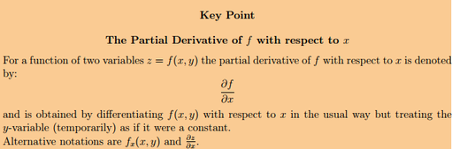
Key Point

The Partial Derivative of $f$ with respect to $x$

For a function of two variables $z = f(x,y)$ the partial derivative of $f$ with respect to $x$ is denoted by

$\frac{\partial f}{\partial x}$

and is obtained by differentiating $f(x,y)$ with respect to $x$ in the usual way but treating the $y$-variable (temporarily) as if it were a constant.

Alternative notations are $f_x(x,y)$ and $\dfrac{\partial z}{\partial x}$.

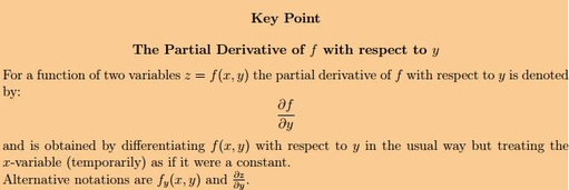
Key Point

The Partial Derivative of $f$ with respect to $y$

For a function of two variables $z = f(x,y)$ the partial derivative of $f$ with respect to $y$ is denoted by

$\frac{\partial f}{\partial y}$

and is obtained by differentiating $f(x,y)$ with respect to $y$ in the usual way but treating the $x$-variable (temporarily) as if it were a constant.

Alternative notations are $f_y(x,y)$ and $\dfrac{\partial z}{\partial y}$.

As we have seen, a function of two variables $f(x,y)$ has two partial derivatives, $\dfrac{\partial f}{\partial x}$ and $\dfrac{\partial f}{\partial y}$. In an exactly analogous way a function of three variables $f(x,y,u)$ will have three partial derivatives $\dfrac{\partial f}{\partial x}$, $\dfrac{\partial f}{\partial y}$ and $\dfrac{\partial f}{\partial u}$ and so on for functions of more than three variables. Each partial derivative is obtained in the same way:

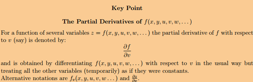
Key Point

The Partial Derivatives of $f(x, y, u, v, w, \ldots)$

For a function of several variables $z = f(x, y, u, v, w, \ldots)$ the partial derivative of $f$ with respect to $v$ (say) is denoted by

$\frac{\partial f}{\partial v}$

and is obtained by differentiating $f(x, y, u, v, w, \ldots)$ with respect to $v$ in the usual way but treating all the other variables (temporarily) as if they were constants.

Alternative notations are $f_v(x, y, u, v, w, \ldots)$ and $\dfrac{\partial f}{\partial v}$.

Example 2.1

Find the partial derivative of $f$ with respect to $x$ and $y$.

(i) $f(x, y) = x^2 y^3$

Solution

$f_x(x, y) = f_x = \frac{\partial f}{\partial x} = 2xy^3$

$f_y(x, y) = f_y = \frac{\partial f}{\partial y} = 3x^2 y^2$

(ii) $f(x, y) = x e^{xy}$

Solution

$f_x(x, y) = f_x = \frac{\partial f}{\partial x} = e^{xy} + xye^{xy}$

$f_y(x, y) = f_y = \frac{\partial f}{\partial y} = x^2 e^{xy}$

2.2 Higher Order Partial Derivatives

Just as we had higher order derivatives with functions of one variable, we will also have higher order derivatives of functions of more than one variable. However, this time we will have more options since we do have more than one variable.

Consider the case of a function of two variables, $f(x,y)$. Since both of the first order partial derivatives are also functions of $x$ and $y$ we could in turn differentiate each with respect to $x$ or $y$. This means that for the case of a function of two variables there will be a total of four possible second order derivatives. Here they are and the notations that we'll use to denote them.

$(f_x)_x = f_{xx} = \frac{\partial}{\partial x}\left(\frac{\partial f}{\partial x}\right) = \frac{\partial^2 f}{\partial x^2}$

$(f_x)_y = f_{xy} = \frac{\partial}{\partial y}\left(\frac{\partial f}{\partial x}\right) = \frac{\partial^2 f}{\partial y \partial x}$

$(f_y)_x = f_{yx} = \frac{\partial}{\partial x}\left(\frac{\partial f}{\partial y}\right) = \frac{\partial^2 f}{\partial x \partial y}$

$(f_y)_y = f_{yy} = \frac{\partial}{\partial y}\left(\frac{\partial f}{\partial y}\right) = \frac{\partial^2 f}{\partial y^2}$

The second and third second order partial derivatives are often called mixed partial derivatives since we are taking derivatives with respect to more than one variable. Note as well that the order that we take the derivatives in is given by the notation for each of these. If we are using the subscripting notation, e.g. $f_{xy}$, then we will differentiate from left to right. In other words, in this case, we will differentiate first with respect to $x$ and then with respect to $y$. With the fractional notation, e.g. $\dfrac{\partial^2 f}{\partial y \partial x}$, it is the opposite. In these cases we differentiate moving along the denominator from right to left. So, again, in this case we differentiate with respect to $x$ first and then $y$.

Example 2.2

Find all the second order derivatives for

$f(x, y) = x^4 y^2 - x^2 y^6$

Solution

$\frac{\partial f}{\partial x} = 4x^3 y^2 - 2xy^6$

$\frac{\partial f}{\partial y} = 2x^4 y - 6x^2 y^5$

$\frac{\partial^2 f}{\partial x^2} = 12x^2 y^2 - 2y^6$

$\frac{\partial^2 f}{\partial y^2} = 2x^4 - 30x^2 y^4$

$\frac{\partial^2 f}{\partial y \partial x} = 8x^3 y - 12xy^5$

$\frac{\partial^2 f}{\partial x \partial y} = 8x^3 y - 12xy^5$

We prove that the mixed partial derivatives $\dfrac{\partial^2 f}{\partial y \partial x}$ and $\dfrac{\partial^2 f}{\partial x \partial y}$ are equal at points where both are continuous. This goes under several different names including "equality of mixed partials" and "Clairaut's theorem".

So far we have only looked at second order derivatives. There are, of course, higher order derivatives as well. Here are a couple of the third order partial derivatives of a function of two variables.

$f_{xyx} = (f_{xy})_x = \frac{\partial}{\partial x}\left(\frac{\partial^2 f}{\partial y \partial x}\right) = \frac{\partial^3 f}{\partial x \partial y \partial x}$

$f_{yxx} = (f_{yx})_x = \frac{\partial}{\partial x}\left(\frac{\partial^2 f}{\partial x \partial y}\right) = \frac{\partial^3 f}{\partial x^2 \partial y}$

Notice as well that for both of these we differentiate once with respect to $y$ and twice with respect to $x$. There is also another third order partial derivative in which we can do this, $f_{xxy}$.

2.3 Composite Function

Composite function is a function where one function is inside of another function. We need to use chain rule to differentiate composite of functions.

Recall the chain rule for ordinary derivatives: if $y = f(u)$ and $u = g(x)$ then

$\frac{dy}{dx} = \frac{dy}{du}\frac{du}{dx}$

In the above we call $u$ the intermediate variable and $x$ the independent variable.

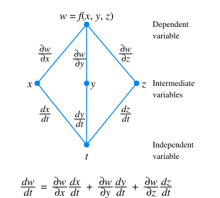
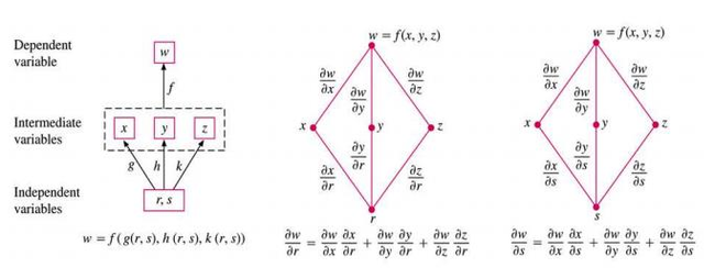
For partial derivatives the chain rule is more complicated. It depends on how many intermediate variables and how many independent variables are present. Below three theorems are given which it is hoped indicate the general points. Essentially, every intermediate variable has to have a term corresponding to it in the right hand side of the chain rule formula. For example in the second theorem below there are three intermediate variables $x$, $y$ and $z$ and three terms in the RHS.

Theorem 1: Chain rule for functions of two independent variables

Theorem 2: Chain rule for functions of three independent variables

Theorem 3: Chain rule for two independent variables and three intermediate variables

$\frac{\partial w}{\partial s} = \frac{\partial w}{\partial x}\frac{\partial x}{\partial s} + \frac{\partial w}{\partial y}\frac{\partial y}{\partial s} + \frac{\partial w}{\partial z}\frac{\partial z}{\partial s}$

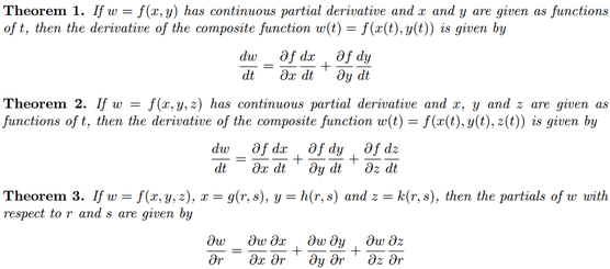
To summarize,

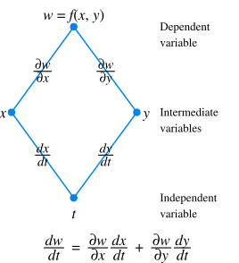
Theorem 1. If $w = f(x, y)$ has continuous partial derivatives and $x$ and $y$ are given as functions of $t$, then the derivative of the composite function $w(t) = f(x(t), y(t))$ is given by

$\frac{dw}{dt} = \frac{\partial f}{\partial x}\frac{dx}{dt} + \frac{\partial f}{\partial y}\frac{dy}{dt}$

Theorem 2. If $w = f(x, y, z)$ has continuous partial derivatives and $x$, $y$ and $z$ are given as functions of $t$, then the derivative of the composite function $w(t) = f(x(t), y(t), z(t))$ is given by

$\frac{dw}{dt} = \frac{\partial f}{\partial x}\frac{dx}{dt} + \frac{\partial f}{\partial y}\frac{dy}{dt} + \frac{\partial f}{\partial z}\frac{dz}{dt}$

Theorem 3. If $w = f(x, y, z)$, $x = g(r, s)$, $y = h(r, s)$ and $z = k(r, s)$, then the partials of $w$ with respect to $r$ and $s$ are given by

$\frac{\partial w}{\partial r} = \frac{\partial w}{\partial x}\frac{\partial x}{\partial r} + \frac{\partial w}{\partial y}\frac{\partial y}{\partial r} + \frac{\partial w}{\partial z}\frac{\partial z}{\partial r}$

Example 2.3

(i) Let $F = f(x, y) = xy + 2y$ and $x = t$, $y = e^{-t}$. Calculate $dF/dt$ using the chain rule.

Solution

$\frac{dF}{dt} = \left(\frac{\partial f}{\partial x}\right)\frac{dx}{dt} + \left(\frac{\partial f}{\partial y}\right)\frac{dy}{dt}$

$= y\frac{dx}{dt} + (x + 2)\frac{dy}{dt}$

$= e^{-t}(1) + (t + 2)(-e^{-t})$

(ii) Let $F = f(x, y) = x^3 - xy + y^3$ and $x = r\cos\theta$, $y = r\sin\theta$. Calculate $dF/dr$ and $dF/d\theta$.

Solution

$\frac{dF}{dr} = \left(\frac{\partial f}{\partial x}\right)\frac{\partial x}{\partial r} + \left(\frac{\partial f}{\partial y}\right)\frac{\partial y}{\partial r}$

$\frac{dF}{dr} = (3x^2 - y)\cos\theta + (-x + 3y^2)\sin\theta$

$\frac{dF}{dr} = 3r^2(\cos^3\theta + \sin^3\theta) - 2r\cos\theta\sin\theta$

$\frac{dF}{d\theta} = \left(\frac{\partial f}{\partial x}\right)\frac{\partial x}{\partial \theta} + \left(\frac{\partial f}{\partial y}\right)\frac{\partial y}{\partial \theta}$

$\frac{dF}{d\theta} = (3x^2 - y)(-r\sin\theta) + (-x + 3y^2)r\cos\theta$

$\frac{dF}{d\theta} = 3r^3(\sin\theta - \cos\theta)\cos\theta\sin\theta + r^2(\sin^2\theta - \cos^2\theta)$

(iii) Let $F = f(x, y, z) = xy + z$ and $x = \cos t$, $y = \sin t$ and $z = t$. Calculate $dF/dt$.

Solution

$\frac{dF}{dt} = \frac{\partial F}{\partial x}\frac{\partial x}{\partial t} + \frac{\partial F}{\partial y}\frac{\partial y}{\partial t} + \frac{\partial F}{\partial z}\frac{\partial z}{\partial t}$

$= y(-\sin t) + x(\cos t) + (1)(1)$

$= -\sin^2 t + \cos^2 t + 1$

(iv) What rate is the area of a rectangle changing if its length is 15 m and increasing at 3 ms$^{-1}$ while its width is 6 m and increasing at 2 ms$^{-1}$?

Solution

Let $x$ be the length, $y$ the width, $A$ the area and $t =$ time. The information given tells us that

$\frac{dx}{dt} = 3 \text{ ms}^{-1}, \qquad \frac{dy}{dt} = 2 \text{ ms}^{-1}.$

Obviously $A = xy$. We want $dA/dt$ when $x = 15$ and $y = 6$. This is given by the chain rule as follow:

$\frac{dA}{dt} = \frac{\partial A}{\partial x}\frac{dx}{dt} + \frac{\partial A}{\partial y}\frac{dy}{dt} = y\frac{dx}{dt} + x\frac{dy}{dt} = (6)(3) + (15)(2) = 48 \text{ m}^2\text{s}^{-1}$

2.4 Implicit Function

The chain rule can also be used to derive a simpler method for finding the derivative of an implicitly defined function.

Suppose that $F(x,y) = 0$ defines $y$ as an implicit function of $x$ we will call $y = f(x)$. We wish to find $dy/dx$. We do so by differentiating both sides of $F(x,y) = 0$ with respect to $x$. To differentiate the left side with respect to $x$, $F(x,y)$, we will use the chain rule, remembering that $F(x,y) = F(x,f(x))$. So, $F$ is ultimately a function of $x$.

$\frac{dF}{dx} = \left(\frac{\partial f}{\partial x}\right)\frac{dx}{dx} + \left(\frac{\partial f}{\partial y}\right)\frac{dy}{dx}$

$\frac{dF}{dx} = \left(\frac{\partial f}{\partial x}\right) + \left(\frac{\partial f}{\partial y}\right)\frac{dy}{dx}$

$0 = \left(\frac{\partial f}{\partial x}\right) + \left(\frac{\partial f}{\partial y}\right)\frac{dy}{dx}$

$\frac{dy}{dx} = -\frac{\partial f/\partial x}{\partial f/\partial y}$

Example 2.4

Find $dy/dx$ if

(i) $2xy - y^3 + 1 - x - 2y = 0$

Solution

$f(x,y) = 2xy - y^3 + 1 - x - 2y$

$\frac{dy}{dx} = -\frac{\partial f/\partial x}{\partial f/\partial y}$

$= \frac{2y - 1}{2x - 3y^2 - 2}$

(ii) $x - x^2 y^3 = 0$

Solution

$f(x,y) = x - x^2y^3$

$\frac{dy}{dx} = -\frac{1 - 2xy^3}{-3x^2y^2}$

Now suppose $z$ is given implicitly as a function $z = z(x,y)$ by an equation of the form $f(x,y,z) = 0$. By chain rule, we can get partial derivatives of:

$\frac{\partial z}{\partial x} = -\frac{\partial f/\partial x}{\partial f/\partial z}$

$\frac{\partial z}{\partial y} = -\frac{\partial f/\partial y}{\partial f/\partial z}$

2.5 Partial Derivatives Using Jacobian

Example 2.5(ii) may be viewed as an example of transformation of coordinates. Consider the transformation or mapping from the $(x,y)$ plane to the $(u,v)$ plane defined by

$u = u(x,y), \qquad v = v(x,y)$

Then a function $F = f(x,y)$ of $x$ and $y$ becomes a function $F = T(u,v)$ of $u$ and $v$ under the transformation, and the partial derivatives are related by the chain rule:

$\frac{\partial F}{\partial x} = \frac{\partial F}{\partial u}\frac{\partial u}{\partial x} + \frac{\partial F}{\partial v}\frac{\partial v}{\partial x}$

$\frac{\partial F}{\partial y} = \frac{\partial F}{\partial u}\frac{\partial u}{\partial y} + \frac{\partial F}{\partial v}\frac{\partial v}{\partial y}$

In matrix notation this becomes

$\begin{bmatrix} \dfrac{\partial F}{\partial x} \\ \dfrac{\partial F}{\partial y} \end{bmatrix} = \begin{bmatrix} \dfrac{\partial u}{\partial x} & \dfrac{\partial v}{\partial x} \\ \dfrac{\partial u}{\partial y} & \dfrac{\partial v}{\partial y} \end{bmatrix} \begin{bmatrix} \dfrac{\partial F}{\partial u} \\ \dfrac{\partial F}{\partial v} \end{bmatrix}$

The determinant of the matrix of the transformation is called the Jacobian of the transformation and is abbreviated to

$\frac{\partial(u,v)}{\partial(x,y)} \qquad \text{or simply to} \qquad J$

So that

$J = \frac{\partial(u,v)}{\partial(x,y)} = \begin{vmatrix} \dfrac{\partial u}{\partial x} & \dfrac{\partial v}{\partial x} \\ \dfrac{\partial u}{\partial y} & \dfrac{\partial v}{\partial y} \end{vmatrix} = \begin{vmatrix} u_x & v_x \\ u_y & v_y \end{vmatrix}$

The matrix itself is referred to as the Jacobian matrix. The Jacobian plays an important role in various applications of mathematics in engineering, particularly in implementing changes in variables in multiple integrals.

We can also have $x = X(u,v)$ and $y = Y(u,v)$ which represent a transformation of the $(u,v)$ plane into the $(x,y)$ plane. This is called the inverse transformation and we can relate the partial derivatives by

$\frac{\partial F}{\partial u} = \frac{\partial F}{\partial x}\frac{\partial x}{\partial u} + \frac{\partial F}{\partial y}\frac{\partial y}{\partial u}$

$\frac{\partial F}{\partial v} = \frac{\partial F}{\partial x}\frac{\partial x}{\partial v} + \frac{\partial F}{\partial y}\frac{\partial y}{\partial v}$

The Jacobian of this inverse transformation is

$J_1 = \frac{\partial(x,y)}{\partial(u,v)} = \begin{vmatrix} x_u & y_u \\ x_v & y_v \end{vmatrix}$

And, provided $J \neq 0$, it is always true that $J_1 = J^{-1}$ or

$\frac{\partial(x,y)}{\partial(u,v)}\frac{\partial(u,v)}{\partial(x,y)} = 1$

If $J = 0$ then the variables $u$ and $v$ are functionally dependent; that is, a relationship of the form $f(u,v) = 0$ exists. This implies a non-unique correspondence between points in the $(x,y)$ and $(u,v)$ planes.

Example 2.5

(i) Obtain the Jacobian $J$ of the transformation $u=(2x-y)/2$ and $v=y/2$. Determine the inverse transformation and obtain $J_1$. Show that $J_1 = J^{-1}$.

Solution

$J = \frac{\partial(u,v)}{\partial(x,y)} = \begin{vmatrix} 1 & -\frac{1}{2} \\ 0 & \frac{1}{2} \end{vmatrix} = \frac{1}{2}$

Re-arranging, $x = u + v$ and $y = 2v$, therefore

$J_1 = \frac{\partial(x,y)}{\partial(u,v)} = \begin{vmatrix} 1 & 1 \\ 0 & 2 \end{vmatrix} = 2 \qquad \text{(shown)}$

(ii) If $x = r \cos\theta$, $y = r \sin\theta$; evaluate $J_1 = \dfrac{\partial(x,y)}{\partial(r,\theta)}$ and the inverse $J^{-1} = \dfrac{\partial(r,\theta)}{\partial(x,y)}$. Show that $J_1 = J^{-1}$.

Solution

$\frac{\partial(x,y)}{\partial(r,\theta)} = \begin{vmatrix} \dfrac{\partial x}{\partial r} & \dfrac{\partial x}{\partial \theta} \\ \dfrac{\partial y}{\partial r} & \dfrac{\partial y}{\partial \theta} \end{vmatrix} = \begin{vmatrix} \cos\theta & -r\sin\theta \\ \sin\theta & r\cos\theta \end{vmatrix} = r\cos^2\theta + r\sin^2\theta = r$

Re-arranging, $r^2 = x^2 + y^2$, $\theta = \tan^{-1}(y/x)$

$\frac{\partial(r,\theta)}{\partial(x,y)} = \begin{vmatrix} \dfrac{\partial r}{\partial x} & \dfrac{\partial r}{\partial y} \\ \dfrac{\partial \theta}{\partial x} & \dfrac{\partial \theta}{\partial y} \end{vmatrix} = \begin{vmatrix} \dfrac{x}{r} & \dfrac{y}{r} \\ -\dfrac{y}{r^2} & \dfrac{x}{r^2} \end{vmatrix} = \frac{x^2}{r^3} + \frac{y^2}{r^3} = \frac{x^2 + y^2}{r^3} = \frac{r^2}{r^3} = \frac{1}{r} \qquad \text{(shown)}$

2.6 Total Differential

Partial derivatives occur in the mathematical modelling of many engineering problems; this leads to the study of partial differential equations. Partial differentiation is also a tool for the analysis of many practical problems.

The total differential of the function of two variables $(x,y)$ defined by $F = f(x,y)$ is given by

$dF = \frac{\partial f}{\partial x}dx + \frac{\partial f}{\partial y}dy$

Differential $dF$ is an approximation to change $\Delta F$ in $F = f(x,y)$ resulting from small changes $\Delta x$ and $\Delta y$ in the independent variables $x$ and $y$, i.e.

$\Delta F \approx \frac{\partial f}{\partial x}\Delta x + \frac{\partial f}{\partial y}\Delta y$

This extends to functions of as many variables as we please, provided that the partial derivatives exist. For example, for a function of three variables $(x,y,z)$ defined by $F = f(x,y,z)$, we have

$dF = \frac{\partial f}{\partial x}dx + \frac{\partial f}{\partial y}dy + \frac{\partial f}{\partial z}dz$

And thus

$\Delta F \approx \frac{\partial f}{\partial x}\Delta x + \frac{\partial f}{\partial y}\Delta y + \frac{\partial f}{\partial z}\Delta z$

The total differential therefore shows the variation of the function with respect to small changes in all the independent variables.

Example 2.6

Compute the total differential for the function $F = x^y$.

Solution

$dF = yx^{y-1}dx + x^y \ln x\, dy$

All physical measurements are subjected to error, and a calculated quantity usually depends on several measurements. It is very important to know the degree of accuracy that can be relied upon in a quantity that has been calculated. The total differential can be used to estimate error bounds for quantities calculated from experimental results or from data that is subject to errors. This is illustrated in example 2.7.

Example 2.7

The volume of a circular cylinder of radius $r$ and height $h$ is given by $V = \pi r^2 h$. If $r = 3$ cm subject to an error of 0.01 cm and $h = 5$ cm subject to an error of 0.005 cm, find the greatest possible error in the calculation of $V$.

Solution

The total differential is

$\Delta V \approx \frac{\partial V}{\partial r}dr + \frac{\partial V}{\partial h}dh = 2\pi rh\,dr + \pi r^2 dh$

$\Delta V \approx \pi r(2h\Delta r + r\Delta h)$

When $r = 3$ and $h = 5$, we are given that $dr = 0.01$ and $dh = 0.005$, so that

$\Delta V \approx 3\pi(10 \times 0.01 + 3 \times 0.005) = 0.345\pi$

Example 2.8

A balloon is in the form of right circular cylinder of radius 1.5 m and length 4 m and is surrounded by hemispherical ends. If the radius is increased by 0.01 m and the length by 0.05 m, find the percentage change in the volume of the balloon.

Solution

Volume of balloon = volume of cylinder + volume of 2 hemispheres

$V = \pi r^2 h + (2/3)\pi r^3 + (2/3)\pi r^3 = \pi r^2 h + (4/3)\pi r^3$

$\Delta V \approx \frac{\partial V}{\partial r}dr + \frac{\partial V}{\partial h}dh$

$\Delta V \approx 2\pi rh\,dr + 4\pi r^2 dr + \pi r^2 dh$

When $r = 1.5$ and $h = 4$, $dr = 0.01$ and $dh = 0.05$, hence

$\Delta V \approx 2(1.5)\pi(4)(0.01) + 4\pi(1.5)^2(0.01) + \pi(1.5)^2(0.05) = 0.3225\pi = 1.013$

% change in volume $= 100 \times (1.013/V) = 100 \times (1.013/42.411) = 2.39\%$

2.7 Tangent Planes and Normal to Surfaces in Three Dimensions

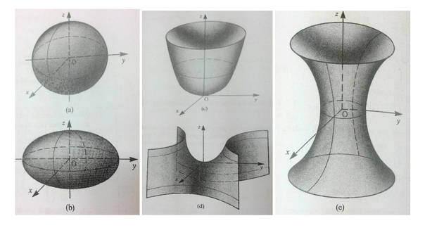
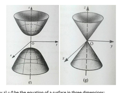
The circle, ellipse, hyperbola and parabola of two dimensions generalize in three dimensions to give the sphere, ellipsoid, hyperboloid and paraboloid as illustrated. Equations of these surfaces are as follow:

(a) Sphere: $x^2 + y^2 + z^2 = r^2$

(b) Ellipsoid: $\dfrac{x^2}{a^2} + \dfrac{y^2}{b^2} + \dfrac{z^2}{c^2} = 1$

(c) Elliptic paraboloid: $\dfrac{x^2}{a^2} + \dfrac{y^2}{b^2} = cz$

(d) Hyperbolic paraboloid: $\dfrac{y^2}{b^2} - \dfrac{x^2}{a^2} = cz$

(e) Hyperboloid of one sheet: $\dfrac{x^2}{a^2} + \dfrac{y^2}{b^2} - \dfrac{z^2}{c^2} = 1$

(f) Hyperboloid of two sheets: $\dfrac{x^2}{a^2} + \dfrac{y^2}{b^2} - \dfrac{z^2}{c^2} = -1$

(g) Elliptic cone: $\dfrac{x^2}{a^2} + \dfrac{y^2}{b^2} - \dfrac{z^2}{c^2} = 0$

In general, let $f(x,y,z) = 0$ be the equation of a surface in three dimensions:

$df = \frac{\partial f}{\partial x}dx + \frac{\partial f}{\partial y}dy + \frac{\partial f}{\partial z}dz = 0$

Interpreting this geometrically, we can say that if $P$ is the point $(x,y,z)$ and $Q$ is the point $(x + dx, y + dy, z + dz)$ then $PQ$ is a tangent line to the surface. Since the equation before implies that the scalar product

$\left(\frac{\partial f}{\partial x}, \frac{\partial f}{\partial y}, \frac{\partial f}{\partial z}\right) \cdot (dx, dy, dz) = 0$

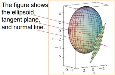
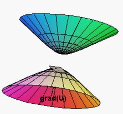
we deduce that the vector $(dx,dy,dz)$ is perpendicular to the vector $(\partial f/\partial x, \partial f/\partial y, \partial f/\partial z)$. Therefore all the tangent lines to the surface at $P$ are perpendicular to the vector $(\partial f/\partial x, \partial f/\partial y, \partial f/\partial z)$. Hence, the equation of the tangent plane to the surface at the point $(x_0,y_0,z_0)$ on the surface is given by:

$(x - x_0)\left(\frac{\partial f}{\partial x}\right)_0 + (y - y_0)\left(\frac{\partial f}{\partial y}\right)_0 + (z - z_0)\left(\frac{\partial f}{\partial z}\right)_0 = 0$

Where

$\left(\frac{\partial f}{\partial x}\right)_0 = f_x(x_0, y_0, z_0), \qquad \text{and so on}$

The equation of the normal at the point $(x_0,y_0,z_0)$ is:

$\frac{x - x_0}{\left(\frac{\partial f}{\partial x}\right)_0} = \frac{y - y_0}{\left(\frac{\partial f}{\partial y}\right)_0} = \frac{z - z_0}{\left(\frac{\partial f}{\partial z}\right)_0}$

Example 2.9

Find the tangent plane to $x^2 + y^2 + z - 9 = 0$ at $(1,2,4)$.

Solution

Determining the slopes of the tangent plane,

$\frac{\partial f}{\partial x} = 2x, \qquad \frac{\partial f}{\partial y} = 2y, \qquad \frac{\partial f}{\partial z} = 1$

$\left(\frac{\partial f}{\partial x}\right)_{(1,2,4)} = 2, \qquad \left(\frac{\partial f}{\partial y}\right)_{(1,2,4)} = 4, \qquad \left(\frac{\partial f}{\partial z}\right)_{(1,2,4)} = 1$

The equation of the tangent plane is therefore:

$2(x-1) + 4(y-2) + (z-4) = 0 \qquad \text{or} \qquad 2x + 4y + z = 14$

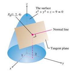
The dotted lines are the $x$, $y$, $z$ tangent lines. They lie in the plane. All tangent lines lie in the tangent plane. These particular lines are tangent to the 'partial functions' – where $z$ is fixed at $z_0 = 4$, $y$ is fixed at $y_0 = 2$ and $x$ is fixed at $x_0 = 1$. The plane is balancing on the surface and touching at the tangent point.

The equation of normal line in parametric form:

$x = x_0 + 2t, \qquad y = y_0 + 4t, \qquad z = z_0 + t$

So, at $(1,2,4)$,

$x = 1 + 2t, \qquad y = 2 + 4t, \qquad z = 4 + t$

Therefore, the symmetric equation of the normal at the point $(1,2,4)$ is:

$\frac{x-1}{2} = \frac{y-2}{4} = \frac{z-4}{1}$

The normal vector $N$ has components 2, 4, 1. Starting from $(1,2,4)$ the line goes out along $N$-perpendicular to the plane and the surface, as shown in the figure above.

Example 2.10

Find the tangent plane and normal line to the ellipsoid $x^2/4 + y^2 + z^2/9 = 3$ at point $(-2,1,-3)$.

Solution

$\frac{\partial f}{\partial x} = \frac{x}{2}, \qquad \frac{\partial f}{\partial y} = 2y, \qquad \frac{\partial f}{\partial z} = \frac{2z}{9}$

At point $(-2,1,-3)$,

$\left(\frac{\partial f}{\partial x}\right)_{(-2,1,-3)} = -1, \qquad \left(\frac{\partial f}{\partial y}\right)_{(-2,1,-3)} = 2, \qquad \left(\frac{\partial f}{\partial z}\right)_{(-2,1,-3)} = \frac{-2}{3}$

Thus, the equation of the tangent plane at $(-2,1,-3)$ is:

$-1(x+2) + 2(y-1) - \frac{2}{3}(z+3) = 0 \qquad \text{or} \qquad 3x - 6y + 2z + 18 = 0$

The normal line at $(-2,1,-3)$ is therefore:

$\frac{x + 2}{-1} = \frac{y - 1}{2} = \frac{z + 3}{-\frac{2}{3}}$

The figure shows the ellipsoid, tangent plane, and normal line.

Example 2.11

Find the equation of tangent plane to the hyperboloid in 2 sheets $x^2 - y^2 - z^2 = 4$ at the point $(3,2,1)$.

Solution

$\frac{\partial f}{\partial x} = 2x, \qquad \frac{\partial f}{\partial y} = -2y, \qquad \frac{\partial f}{\partial z} = -2z$

At point $(3,2,1)$,

$\frac{\partial f}{\partial x} = 6, \qquad \frac{\partial f}{\partial y} = -4, \qquad \frac{\partial f}{\partial z} = -2$

The equation of tangent plane:

$6(x - 3) - 4(y - 2) - 2(z - 1) = 0$

$z = 3x - 2y - 4$

Example 2.12

Find an equation of the tangent plane at the point $\left(\dfrac{-15}{\sqrt{17}}, \dfrac{15}{\sqrt{17}}, 2\right)$ on a power plant's cooling tower that is part of the hyperboloid of one sheet

$\frac{x^2}{5^2} + \frac{y^2}{3^2} - \frac{z^2}{2^2} = 1$

Solution

$\frac{\partial f}{\partial x} = \frac{2}{25}x, \qquad \frac{\partial f}{\partial y} = \frac{2y}{9}, \qquad \frac{\partial f}{\partial z} = \frac{-z}{2}$

At point $\left(\dfrac{-15}{\sqrt{17}}, \dfrac{15}{\sqrt{17}}, 2\right)$,

$\frac{\partial f}{\partial x} = \frac{-6}{5\sqrt{17}}, \qquad \frac{\partial f}{\partial y} = \frac{10}{3\sqrt{17}}, \qquad \frac{\partial f}{\partial z} = -1$

Thus, the equation of tangent plane:

$\frac{-6}{5\sqrt{17}}\left(x + \frac{15}{\sqrt{17}}\right) + \frac{10}{3\sqrt{17}}\left(y - \frac{15}{\sqrt{17}}\right) - 1(z - 2) = 0$

$\frac{-6}{5\sqrt{17}}x - \frac{90}{5(17)} + \frac{10}{3\sqrt{17}}y - \frac{50}{17} - z + 2 = 0$

$\frac{-6}{5\sqrt{17}}x + \frac{10}{3\sqrt{17}}y - 2 - z = 0$

$-18x + 50y - 30\sqrt{17} - 15\sqrt{17}z = 0$

$18x - 50y + 15\sqrt{17}z = -30\sqrt{17}$