Lecture 3: Vector Algebra I

Note: The lecture notes here are from Session 2022/2023.

Download the original PDF →


3.1 Introduction​

In the world of engineering, physical quantities can be divided mainly into scalar and vector. These quantities can be represented by numbers alone (i.e., magnitude only), with the appropriate units, and they are called scalars. Another physical quantity with magnitude and direction are called vectors. Scalars and vectors are the underlying elements in vector analysis.

Scalar vs Vector​

ScalarVector
ExampleMass; length; temperature; voltageDisplacement; velocity; force; acceleration
Unit of quantitieskg; m; Degree; Voltm; ms−1\text{ms}^{-1}; N; ms−2\text{ms}^{-2}
DirectionNoYes
Symbol/Notationaa; bb; AA; BB; PQPQa∼\underset{\sim}{a}; b∼\underset{\sim}{b}; OA→\overrightarrow{OA}, OB→\overrightarrow{OB}, PQ→\overrightarrow{PQ}

3.2 Basic Concepts​

A scalar is a quantity that is determined by its magnitude. It takes on a numerical value, i.e., a number. Examples of scalars are time, temperature, length, distance, speed, density, energy, and voltage.

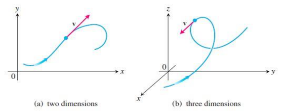
A vector is a quantity that has both magnitude and direction. We can say that a vector is an arrow or a directed line segment. For example, a velocity vector has length or magnitude, which is speed, and direction, which indicates the direction of motion (Fig 3.1); a force vector points in the direction in which the force acts and its length is a measure of the force's strength.

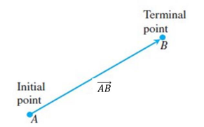
A vector (arrow) has a tail, called its initial point, and a tip, called its terminal point. The length of the arrow equals the distance between initial point and terminal point (Fig 3.1). This is called the length (or magnitude) of the vector a\mathbf{a} and is denoted by ∣a∣|\mathbf{a}|. Another name for length is norm (or Euclidean norm). A vector of length 1 is called a unit vector.

DEFINITIONS

The vector represented by the directed line segment AB→\overrightarrow{AB} has initial point AA and terminal point BB and its length is denoted by ∣AB→∣|\overrightarrow{AB}|. Two vectors are equal if they have the same length and direction.

Fig 3.1: The directed line segment AB is called a vector

Fig 3.1: The directed line segment AB is called a vector
DEFINITION

If v\mathbf{v} is a two-dimensional vector in the plane equal to the vector with initial point at the origin and terminal point (v1,v2)(v_1, v_2), then the component form of v\mathbf{v} is

v=⟨v1,v2⟩.\mathbf{v} = \langle v_1, v_2 \rangle.

If v\mathbf{v} is a three-dimensional vector equal to the vector with initial point at the origin and terminal point (v1,v2,v3)(v_1, v_2, v_3), then the component form of v\mathbf{v} is

v=⟨v1,v2,v3⟩.\mathbf{v} = \langle v_1, v_2, v_3 \rangle.

Fig 3.2: The velocity vector of a particle moving along a path (a) in the plane (b) in space

Fig 3.2: The velocity vector of a particle moving along a path (a) in the plane (b) in space. The arrowhead on the path indicates the direction of motion of the particle.

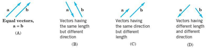
Equality of Vectors - Two vectors a\mathbf{a} and b\mathbf{b} are equal, written a=b\mathbf{a} = \mathbf{b}, if they have the same length and the same direction as shown in Fig. 3.3.

Fig. 3.3 (A) Equal Vectors. (B) – (D) Different Vectors

Fig. 3.3 (A) Equal Vectors. (B) – (D) Different Vectors

3.2.1 Components of a Vector​

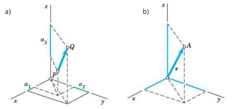
Let a\mathbf{a} be a given vector with initial point PP: (x1,y1,z1)(x_1, y_1, z_1) and terminal point QQ: (x2,y2,z2)(x_2, y_2, z_2). Then the three coordinate differences

a1=x2−x1,a2=y2−y1,a3=z2−z1a_1 = x_2 - x_1, \qquad a_2 = y_2 - y_1, \qquad a_3 = z_2 - z_1

are called the components of the vector a\mathbf{a} with respect to that coordinate system, and we write simply a=[a1,a2,a3]\mathbf{a} = [a_1, a_2, a_3]. See Fig 3.4 (a). The length ∣a∣|\mathbf{a}| of a\mathbf{a} can now readily be expressed in terms of components and the Pythagorean Theorem we have

∣a∣=a12+a22+a32.|\mathbf{a}| = \sqrt{a_1^2 + a_2^2 + a_3^2}.

A Cartesian coordinate system being given, the position vector r\mathbf{r} of a point AA: (x,y,z)(x, y, z) is the vector with the origin (0,0,0)(0, 0, 0) as the initial point and AA as the terminal point (See Fig 3.4 (b)).

Fig 3.4 (a) Components of a vector (b) Position vector r of a point A: (x, y, z)

Fig 3.4 (a) Components of a vector (b) Position vector r of a point A: (x, y, z)

Example 3.1: Components and Length of a Vector​

Solution

The vector a\mathbf{a} with initial point PP: (4,0,2)(4, 0, 2) and terminal point QQ: (6,−1,2)(6, -1, 2) has the components

a1=6−4=2,a2=−1−0=−1,a3=2−2=0.a_1 = 6 - 4 = 2, \qquad a_2 = -1 - 0 = -1, \qquad a_3 = 2 - 2 = 0.

Hence a=⟨2,−1,0⟩\mathbf{a} = \langle 2, -1, 0 \rangle

Equation gives the length

∣a∣=22+(−1)2+02=5.|\mathbf{a}| = \sqrt{2^2 + (-1)^2 + 0^2} = \sqrt{5}.

If we choose (−1,5,8)(-1, 5, 8) as the initial point of a\mathbf{a}, the corresponding terminal point is (1,4,8)(1, 4, 8).

If we choose the origin (0,0,0)(0, 0, 0) as the initial point of a\mathbf{a}, the corresponding terminal point is (2,−1,0)(2, -1, 0); its coordinates equal the components of a\mathbf{a}. This suggests that we can determine each point in space by a vector, called the position vector of the point, as follows.

Exercises​

Let u=3i−2j\mathbf{u} = 3\mathbf{i} - 2\mathbf{j} and v=−2i+5j\mathbf{v} = -2\mathbf{i} + 5\mathbf{j}. Find the (a) component form and (b) magnitude (length) of the vector.

  1. 35u+45v\dfrac{3}{5}\mathbf{u} + \dfrac{4}{5}\mathbf{v}
  2. −513u+1213v-\dfrac{5}{13}\mathbf{u} + \dfrac{12}{13}\mathbf{v}

3.2.2 Vector Addition, Scalar Multiplication​

Two principal operations involving vectors are vector addition and scalar multiplication. A scalar is simply a real number, and is called such when we want to draw attention to its differences from vectors. Scalars can be positive, negative, or zero and are used to "scale" a vector by multiplication.

Addition of Vectors

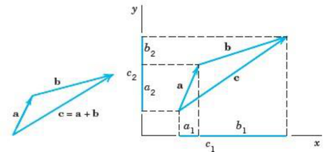
The sum a+b\mathbf{a} + \mathbf{b} of two vectors a=[a1,a2,a3]\mathbf{a} = [a_1, a_2, a_3] and b=[b1,b2,b3]\mathbf{b} = [b_1, b_2, b_3] is obtained by adding the corresponding components,

a+b=[a1+b1,a2+b2,a3+b3].\mathbf{a} + \mathbf{b} = [a_1 + b_1, \quad a_2 + b_2, \quad a_3 + b_3].

Geometrically, place the vectors as in Fig. 3.5 (the initial point of b\mathbf{b} at the terminal point of a\mathbf{a}); then a+b\mathbf{a} + \mathbf{b} is the vector drawn from the initial point of a\mathbf{a} to the terminal point of b\mathbf{b}. Fig. 3.5 also shows (for the plane) that the "algebraic" way and the "geometric" way of vector addition give the same vector.

Fig 3.5 Vector Additions

Fig 3.5 Vector Additions

Basic Properties of Vector Addition​

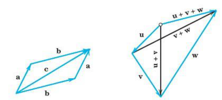
(a) a+b=b+a\mathbf{a} + \mathbf{b} = \mathbf{b} + \mathbf{a} (Commutativity)

(b) (u+v)+w=u+(v+w)(\mathbf{u} + \mathbf{v}) + \mathbf{w} = \mathbf{u} + (\mathbf{v} + \mathbf{w}) (Associativity)

(c) a+0=0+a=a\mathbf{a} + \mathbf{0} = \mathbf{0} + \mathbf{a} = \mathbf{a}

(d) a+(−a)=0.\mathbf{a} + (-\mathbf{a}) = \mathbf{0}.

Properties (a) and (b) are verified geometrically in Fig. 3.6 and Fig 3.7, respectively. Furthermore, −a\mathbf{-a} denotes the vector having the length ∣a∣|\mathbf{a}| and the direction opposite to that of a\mathbf{a}.

Fig 3.6 Commutativity of vector addition. Fig 3.7 Associativity of vector addition

Fig 3.6 Commutativity of vector addition. Fig 3.7 Associativity of vector addition
Scalar Multiplication (Multiplication by a Number)

The product cac\mathbf{a} of any vector a=[a1,a2,a3]\mathbf{a} = [a_1, a_2, a_3] and any scalar cc (real number cc) is the vector obtained by multiplying each component of a\mathbf{a} by cc,

ca=[ca1,ca2,ca3].c\mathbf{a} = [ca_1, ca_2, ca_3].

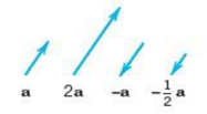
Geometrically, if a≠0\mathbf{a} \neq \mathbf{0} then cac\mathbf{a} with c>0c > 0 has the direction of a\mathbf{a} and with c<0c < 0 the direction opposite to a\mathbf{a}. In any case, the length of cac\mathbf{a} is ∣ca∣=∣c∣ ∣a∣|c\mathbf{a}| = |c|\,|\mathbf{a}|, and ca=0c\mathbf{a} = \mathbf{0} if a=0\mathbf{a} = \mathbf{0} or c=0c = 0 (or both) (See Fig 3.8).

Fig 3.8 Scalar multiplication (multiplication of vectors by scalars (numbers))

Fig 3.8 Scalar multiplication [multiplication of vectors by scalars (numbers)]

Basic Properties of Scalar Multiplication​

From the definitions we obtain directly:

(a) c(a+b)=ca+cbc(\mathbf{a} + \mathbf{b}) = c\mathbf{a} + c\mathbf{b}

(b) (c+k)a=ca+ka(c + k)\mathbf{a} = c\mathbf{a} + k\mathbf{a}

(c) c(ka)=(ck)ac(k\mathbf{a}) = (ck)\mathbf{a} (written ckack\mathbf{a})

(d) 1a=a.1\mathbf{a} = \mathbf{a}.

Example 3.2​

With respect to a given coordinate system, let

a=[4,0,1]andb=[2,−5,13].\mathbf{a} = [4, 0, 1] \qquad \text{and} \qquad \mathbf{b} = \left[2, -5, \tfrac{1}{3}\right].

Solution

Then −a=[−4,0,−1]-\mathbf{a} = [-4, 0, -1], 7a=[28,0,7]7\mathbf{a} = [28, 0, 7], a+b=[6,−5,43]\mathbf{a} + \mathbf{b} = \left[6, -5, \tfrac{4}{3}\right], and

2(a−b)=2[2,5,23]=[4,10,43]=2a−2b.2(\mathbf{a} - \mathbf{b}) = 2\left[2, 5, \tfrac{2}{3}\right] = \left[4, 10, \tfrac{4}{3}\right] = 2\mathbf{a} - 2\mathbf{b}.

Exercises​

Let u=⟨−1,3,1⟩\mathbf{u} = \langle -1, 3, 1 \rangle and v=⟨4,7,0⟩\mathbf{v} = \langle 4, 7, 0 \rangle. Find the components of

(a) 2u+3v2\mathbf{u} + 3\mathbf{v} (b) u−v\mathbf{u} - \mathbf{v} (c) ∣12u∣\left|\dfrac{1}{2}\mathbf{u}\right|.

3.2.3 Unit Vector​

A vector v\mathbf{v} of length 1 is called a unit vector. In this representation, i\mathbf{i}, j\mathbf{j}, k\mathbf{k} are the unit vectors in the positive directions of the axes of a Cartesian coordinate system. The standard unit vectors are

i=⟨1,0,0⟩,j=⟨0,1,0⟩k=⟨0,0,1⟩\mathbf{i} = \langle 1, 0, 0 \rangle, \qquad \mathbf{j} = \langle 0, 1, 0 \rangle \qquad \mathbf{k} = \langle 0, 0, 1 \rangle

Any vector can be written as a linear combination of the standard unit vectors as follows:

v=⟨v1,v2,v3⟩=⟨v1,0,0⟩+⟨0,v2,0⟩+⟨0,0,v3⟩=v1⟨1,0,0⟩+v2⟨0,1,0⟩+v3⟨0,0,1⟩v=v1i+v2j+v3k\begin{aligned} v &= \langle v_1, v_2, v_3 \rangle = \langle v_1, 0, 0 \rangle + \langle 0, v_2, 0 \rangle + \langle 0, 0, v_3 \rangle \\ &= v_1\langle 1, 0, 0 \rangle + v_2\langle 0, 1, 0 \rangle + v_3\langle 0, 0, 1 \rangle \\ v &= v_1\mathbf{i} + v_2\mathbf{j} + v_3\mathbf{k} \end{aligned}

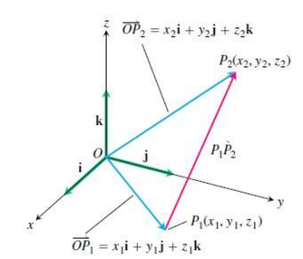
From Figure 3.9, we call the scalar (or number) v1v_1 the i-component of the vector v\mathbf{v}, v2v_2 the j-component, and v3v_3 the k-component. In component form, the vector from P1(x1,y1,z1)P_1(x_1, y_1, z_1) to P2(x2,y2,z2)P_2(x_2, y_2, z_2) is

P1P2→=(x2−x1)i+(y2−y1)j+(z2−z1)k\overrightarrow{P_1P_2} = (x_2 - x_1)\mathbf{i} + (y_2 - y_1)\mathbf{j} + (z_2 - z_1)\mathbf{k}

Fig. 3.9 The vector from P1 to P2 is P1P2

Fig. 3.9 The vector from P₁ to P₂ is P₁P₂

Whenever v≠0\mathbf{v} \neq \mathbf{0}, its length ∣v∣|\mathbf{v}| is not zero and

∣1∣v∣v∣=1∣v∣∣v∣=1\left|\frac{1}{|\mathbf{v}|}\mathbf{v}\right| = \frac{1}{|\mathbf{v}|}|\mathbf{v}| = 1

That is, v/∣v∣\mathbf{v}/|\mathbf{v}| is a unit vector in the direction of v\mathbf{v}, called the direction of the nonzero vector v\mathbf{v}.

Example 3.3​

If v=3i−4j\mathbf{v} = 3\mathbf{i} - 4\mathbf{j} is a velocity vector, express v\mathbf{v} as a product of its speed times a unit vector in the direction of motion.

Solution

Speed is the magnitude (length) of v\mathbf{v}:

∣v∣=(3)2+(−4)2=9+16=5.|\mathbf{v}| = \sqrt{(3)^2 + (-4)^2} = \sqrt{9 + 16} = 5.

The unit vector v/∣v∣\mathbf{v}/|\mathbf{v}| has the same direction as v\mathbf{v}:

v∣v∣=3i−4j5=35i−45j.\frac{\mathbf{v}}{|\mathbf{v}|} = \frac{3\mathbf{i} - 4\mathbf{j}}{5} = \frac{3}{5}\mathbf{i} - \frac{4}{5}\mathbf{j}.

v=3i−4j=5⏟Length(speed)(35i−45j)⏟Direction of motion.\mathbf{v} = 3\mathbf{i} - 4\mathbf{j} = \underbrace{5}_{\substack{\text{Length} \\ \text{(speed)}}}\underbrace{\left(\frac{3}{5}\mathbf{i} - \frac{4}{5}\mathbf{j}\right)}_{\text{Direction of motion}}.

In summary, we can express any nonzero vector v\mathbf{v} in terms of its two important features, length and direction, by writing

v=∣v∣v∣v∣\mathbf{v} = |\mathbf{v}|\frac{\mathbf{v}}{|\mathbf{v}|}

If v≠0\mathbf{v} \neq \mathbf{0}, then

  1. v∣v∣\dfrac{\mathbf{v}}{|\mathbf{v}|} is a unit vector in the direction of v\mathbf{v};
  2. the equation v=∣v∣v∣v∣\mathbf{v} = |\mathbf{v}|\dfrac{\mathbf{v}}{|\mathbf{v}|} expresses v\mathbf{v} as its length times its direction.

Example 3.4​

Find a unit vector u\mathbf{u} in the direction of the vector from P1(1,0,1)P_1(1, 0, 1) to P2(3,2,0)P_2(3, 2, 0).

Solution

We divide P1P2→\overrightarrow{P_1P_2} by its length:

P1P2→=(3−1)i+(2−0)j+(0−1)k=2i+2j−k\overrightarrow{P_1P_2} = (3 - 1)\mathbf{i} + (2 - 0)\mathbf{j} + (0 - 1)\mathbf{k} = 2\mathbf{i} + 2\mathbf{j} - \mathbf{k}

∣P1P2→∣=(2)2+(2)2+(−1)2=4+4+1=9=3|\overrightarrow{P_1P_2}| = \sqrt{(2)^2 + (2)^2 + (-1)^2} = \sqrt{4 + 4 + 1} = \sqrt{9} = 3

u=P1P2→∣P1P2→∣=2i+2j−k3=23i+23j−13k.\mathbf{u} = \frac{\overrightarrow{P_1P_2}}{|\overrightarrow{P_1P_2}|} = \frac{2\mathbf{i} + 2\mathbf{j} - \mathbf{k}}{3} = \frac{2}{3}\mathbf{i} + \frac{2}{3}\mathbf{j} - \frac{1}{3}\mathbf{k}.

The unit vector u\mathbf{u} is the direction of P1P2→\overrightarrow{P_1P_2}.

***PROVE that the length of unit vector is 1.

3.3 Vector in Space​

3.3.1 Cartesian coordinates of a vector in 2D space & its polar expressions​

(a) Definition of a 2D vector​

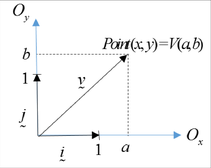
Let OO be the origin and let OxO_x and OyO_y be two mutually perpendicular coordinate axes.

Then, the plane containing OxO_x and OyO_y is called the xy-plane or the xy-coordinate system and OxO_x is called the xx axis and OyO_y is yy axis.

The vector i∼\underset{\sim}{i} is the vector from the origin OO to the point (1,0)(1,0).

The vector j∼\underset{\sim}{j} is the vector from the origin OO to the point (0,1)(0,1).

Note: i∼\underset{\sim}{i} and j∼\underset{\sim}{j} are unit vectors and also position vectors.

A 2D vector from the origin to the point (a, b)

Any vector v∼\underset{\sim}{v} in xy-plane can be represented by v∼=ai∼+bj∼\underset{\sim}{v} = a\underset{\sim}{i} + b\underset{\sim}{j} or v∼=⟨a,b⟩\underset{\sim}{v} = \langle a, b \rangle where aa and bb are scalars. The scalars aa and bb are called the components of the vector v∼\underset{\sim}{v} with respect to that coordinate system.

The vector ai∼a\underset{\sim}{i} and vector bj∼b\underset{\sim}{j} are called the vector components in the direction of i∼\underset{\sim}{i} and j∼\underset{\sim}{j}, respectively.

Notation:

(i) The vector v∼=ai∼+bj∼\underset{\sim}{v} = a\underset{\sim}{i} + b\underset{\sim}{j} can be denoted by v∼=⟨a,b⟩\underset{\sim}{v} = \langle a, b \rangle

(ii) The point PP at (a,b)(a, b) can be denoted by (a,b)(a, b), P(a,b)P(a, b) or P=(a,b)P = (a, b)

(iii) Note that (a,b)≠⟨a,b⟩(a, b) \neq \langle a, b \rangle to avoid confusion. (a,b)(a, b) represent coordinates of a point. ⟨a,b⟩\langle a, b \rangle represent components of a vector.

(b) Vector Algebra of a 2D vector​

Let v1∼=a1i∼+b1j∼\underset{\sim}{v_1} = a_1\underset{\sim}{i} + b_1\underset{\sim}{j} and v2∼=a2i∼+b2j∼\underset{\sim}{v_2} = a_2\underset{\sim}{i} + b_2\underset{\sim}{j} be two vectors. Then

(i) v1∼=v2∼  ⟹  \underset{\sim}{v_1} = \underset{\sim}{v_2} \implies Then, a1=a2a_1 = a_2; b1=b2b_1 = b_2

(ii) v1∼+v2∼  ⟹  \underset{\sim}{v_1} + \underset{\sim}{v_2} \implies Then, (a1+a2)i∼+(b1+b2)j∼(a_1 + a_2)\underset{\sim}{i} + (b_1 + b_2)\underset{\sim}{j}

(iii) v1∼−v2∼  ⟹  \underset{\sim}{v_1} - \underset{\sim}{v_2} \implies Then, (a1−a2)i∼+(b1−b2)j∼(a_1 - a_2)\underset{\sim}{i} + (b_1 - b_2)\underset{\sim}{j}

(iv) Let α\alpha is a scalar, then αv1∼=(αa1)i∼+(αb1)j∼\alpha\underset{\sim}{v_1} = (\alpha a_1)\underset{\sim}{i} + (\alpha b_1)\underset{\sim}{j}

(c) Theorem of an arbitrary vector in 2D space​

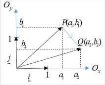
Let PP and QQ be the points (a1,b1)(a_1, b_1) and (a2,b2)(a_2, b_2) respectively. Then, the vector PQ→\overrightarrow{PQ} is given by

PQ→=OQ→−OP→=⟨(a2−a1),(b2−b1)⟩\overrightarrow{PQ} = \overrightarrow{OQ} - \overrightarrow{OP} = \langle (a_2 - a_1), (b_2 - b_1) \rangle

Proof:

Let OP→=⟨a1,b1⟩\overrightarrow{OP} = \langle a_1, b_1 \rangle, OQ→=⟨a2,b2⟩\overrightarrow{OQ} = \langle a_2, b_2 \rangle

PQ→=OQ→−OP→=⟨(a2−a1),(b2−b1)⟩\overrightarrow{PQ} = \overrightarrow{OQ} - \overrightarrow{OP} = \langle (a_2 - a_1), (b_2 - b_1) \rangle

Vector PQ as OQ minus OP

(d) Magnitude & Angle of a vector in 2D space​

Let v∼=ai∼+bj∼\underset{\sim}{v} = a\underset{\sim}{i} + b\underset{\sim}{j} be a 2D vector.

(i) The magnitude of v∼\underset{\sim}{v} is defined as ∣v∼∣=a2+b2|\underset{\sim}{v}| = \sqrt{a^2 + b^2}

(ii) The angle between v∼\underset{\sim}{v} and a line parallel to the x-axis is defined as θ=tan⁡−1ba\theta = \tan^{-1}\dfrac{b}{a}

Hint: Identify the quadrant; θ\theta is positive if it is measured in the direction of anti-clockwise; θ\theta is negative if it is measured in the direction of clockwise.

(e) Transformation of Cartesian form of a 2D vector to polar form​

By using magnitude and angle of a vector, the Cartesian form of a vector (i.e., v∼=ai∼+bj∼\underset{\sim}{v} = a\underset{\sim}{i} + b\underset{\sim}{j}) can be transformed into polar form (i.e., v∼=∣v∼∣⏟magnitude(cos⁡(θ⏟angle)i∼+sin⁡(θ⏟angle)j∼)\underset{\sim}{v} = \underbrace{|\underset{\sim}{v}|}_{\text{magnitude}}(\cos(\underbrace{\theta}_{\text{angle}})\underset{\sim}{i} + \sin(\underbrace{\theta}_{\text{angle}})\underset{\sim}{j}))

Thus, we have v∼=ai∼+bj∼⏟Cartesian domain=∣v∼∣(cos⁡(θ)i∼+sin⁡(θ)j∼)⏟Polar domain\underset{\sim}{v} = \underbrace{a\underset{\sim}{i} + b\underset{\sim}{j}}_{\text{Cartesian domain}} = \underbrace{|\underset{\sim}{v}|(\cos(\theta)\underset{\sim}{i} + \sin(\theta)\underset{\sim}{j})}_{\text{Polar domain}}

Exercise​

(i) Let u∼\underset{\sim}{u}, v∼\underset{\sim}{v} and w∼\underset{\sim}{w} be position vectors of the points U(2,3)U(2,3), V(1,5)V(1,5) and W(3,−4)W(3,-4), respectively. Find

(a) z∼=u∼−2v∼+3w∼\underset{\sim}{z} = \underset{\sim}{u} - 2\underset{\sim}{v} + 3\underset{\sim}{w}

(b) the magnitude of z∼\underset{\sim}{z}

(c) the angle between z∼\underset{\sim}{z} and OxO_x

(d) transform the vector z∼\underset{\sim}{z} from Cartesian domain into Polar domain

(e) compare the result in (a) and (d), explain your finding and relate this in the application of engineering.

(ii) Determine the unit vector in the direction of u∼=2i∼−3j∼\underset{\sim}{u} = 2\underset{\sim}{i} - 3\underset{\sim}{j}

(iii) Find the unit vector from the point P(1,4)P(1,4) to the point Q(3,−5)Q(3,-5)

(iv) Find a vector of magnitude 3 in the direction of v∼=−i∼+3j∼\underset{\sim}{v} = -\underset{\sim}{i} + 3\underset{\sim}{j}

3.3.2 Cartesian coordinates of a vector in 3D space (Volume) & its polar expression​

(a) Definition of a 3D vector​

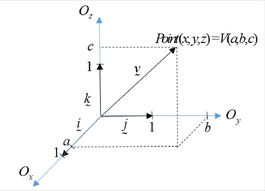
Let OO be the origin and let OxO_x, OyO_y and OzO_z be three mutually perpendicular coordinate axes.

Then, the plane containing OxO_x, OyO_y and OzO_z is called the xyz-plane or the xyz-coordinate system (Follow right hand rule) and OxO_x is called the xx axis, OyO_y is yy axis and OzO_z is zz axis.

The vector i∼\underset{\sim}{i} is the vector from the origin OO to the point (1,0,0)(1,0,0).

The vector j∼\underset{\sim}{j} is the vector from the origin OO to the point (0,1,0)(0,1,0).

The vector k∼\underset{\sim}{k} is the vector from the origin OO to the point (0,0,1)(0,0,1).

Note: i∼\underset{\sim}{i}, j∼\underset{\sim}{j} and k∼\underset{\sim}{k} are unit vectors and also position vectors.

A 3D vector from the origin to the point (a, b, c)

Any vector v∼\underset{\sim}{v} in xyz-plane can be represented by v∼=ai∼+bj∼+ck∼\underset{\sim}{v} = a\underset{\sim}{i} + b\underset{\sim}{j} + c\underset{\sim}{k} or v∼=⟨a,b,c⟩\underset{\sim}{v} = \langle a, b, c \rangle where aa, bb and cc are scalars. The scalars aa, bb and cc are called the components of the vector v∼\underset{\sim}{v} with respect to that coordinate system.

The vector ai∼a\underset{\sim}{i}, vector bj∼b\underset{\sim}{j} and vector ck∼c\underset{\sim}{k} are called the vector components in the direction of i∼\underset{\sim}{i}, j∼\underset{\sim}{j} and k∼\underset{\sim}{k} respectively.

Notation:

(i) The vector v∼=ai∼+bj∼+ck∼\underset{\sim}{v} = a\underset{\sim}{i} + b\underset{\sim}{j} + c\underset{\sim}{k} can be denoted by v∼=⟨a,b,c⟩\underset{\sim}{v} = \langle a, b, c \rangle

(ii) The point PP at (a,b,c)(a, b, c) can be denoted by (a,b,c)(a, b, c), P(a,b,c)P(a, b, c) or P=(a,b,c)P = (a, b, c)

(iii) Note that (a,b,c)≠⟨a,b,c⟩(a, b, c) \neq \langle a, b, c \rangle to avoid confusion. (a,b,c)(a, b, c) represent coordinates of a point. ⟨a,b,c⟩\langle a, b, c \rangle represent components of a vector.

(b) Vector Algebra of a 3D vector​

Let v1∼=a1i∼+b1j∼+c1k∼\underset{\sim}{v_1} = a_1\underset{\sim}{i} + b_1\underset{\sim}{j} + c_1\underset{\sim}{k} and v2∼=a2i∼+b2j∼+c2k∼\underset{\sim}{v_2} = a_2\underset{\sim}{i} + b_2\underset{\sim}{j} + c_2\underset{\sim}{k} be two vectors. Then

(i) v1∼=v2∼  ⟹  \underset{\sim}{v_1} = \underset{\sim}{v_2} \implies Then, a1=a2a_1 = a_2; b1=b2b_1 = b_2; c1=c2c_1 = c_2

(ii) v1∼+v2∼  ⟹  \underset{\sim}{v_1} + \underset{\sim}{v_2} \implies Then, (a1+a2)i∼+(b1+b2)j∼+(c1+c2)k∼(a_1 + a_2)\underset{\sim}{i} + (b_1 + b_2)\underset{\sim}{j} + (c_1 + c_2)\underset{\sim}{k}

(iii) v1∼−v2∼  ⟹  \underset{\sim}{v_1} - \underset{\sim}{v_2} \implies Then, (a1−a2)i∼+(b1−b2)j∼+(c1−c2)k∼(a_1 - a_2)\underset{\sim}{i} + (b_1 - b_2)\underset{\sim}{j} + (c_1 - c_2)\underset{\sim}{k}

(iv) Let α\alpha is a scalar, then αv1∼=(αa1)i∼+(αb1)j∼+(αc1)k∼\alpha\underset{\sim}{v_1} = (\alpha a_1)\underset{\sim}{i} + (\alpha b_1)\underset{\sim}{j} + (\alpha c_1)\underset{\sim}{k}

(c) Theorem of an arbitrary vector in 3D space​

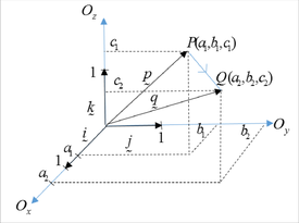
Let PP and QQ be the points (a1,b1,c1)(a_1, b_1, c_1) and (a2,b2,c2)(a_2, b_2, c_2) respectively. Then, the vector PQ→\overrightarrow{PQ} is given by

PQ→=OQ→−OP→=⟨(a2−a1),(b2−b1),(c2−c1)⟩\overrightarrow{PQ} = \overrightarrow{OQ} - \overrightarrow{OP} = \langle (a_2 - a_1), (b_2 - b_1), (c_2 - c_1) \rangle

Proof:

Let OP→=⟨a1,b1,c1⟩\overrightarrow{OP} = \langle a_1, b_1, c_1 \rangle, OQ→=⟨a2,b2,c2⟩\overrightarrow{OQ} = \langle a_2, b_2, c_2 \rangle,

PQ→=OQ→−OP→=⟨(a2−a1),(b2−b1),(c2−c1)⟩\overrightarrow{PQ} = \overrightarrow{OQ} - \overrightarrow{OP} = \langle (a_2 - a_1), (b_2 - b_1), (c_2 - c_1) \rangle

Vector PQ as OQ minus OP in 3D

(d) Magnitude & Angle of a vector in 3D space​

Let v∼=ai∼+bj∼+ck∼\underset{\sim}{v} = a\underset{\sim}{i} + b\underset{\sim}{j} + c\underset{\sim}{k} be a 3D vector and let α\alpha, β\beta, and γ\gamma be the direction angles of v∼=ai∼+bj∼+ck∼\underset{\sim}{v} = a\underset{\sim}{i} + b\underset{\sim}{j} + c\underset{\sim}{k}

The direction angles alpha, beta and gamma of a 3D vector

The magnitude and angle that define vector v∼\underset{\sim}{v} can be obtained as following:

(i) The magnitude of v∼\underset{\sim}{v} is defined as ∣v∼∣=a2+b2+c2|\underset{\sim}{v}| = \sqrt{a^2 + b^2 + c^2}

(ii) The angle between v∼\underset{\sim}{v} and a line parallel to the x-axis is defined as α=cos⁡−1a∣v∼∣\alpha = \cos^{-1}\dfrac{a}{|\underset{\sim}{v}|};

The angle between v∼\underset{\sim}{v} and a line parallel to the y-axis is defined as β=cos⁡−1b∣v∼∣\beta = \cos^{-1}\dfrac{b}{|\underset{\sim}{v}|};

The angle between v∼\underset{\sim}{v} and a line parallel to the z-axis is defined as γ=cos⁡−1c∣v∼∣\gamma = \cos^{-1}\dfrac{c}{|\underset{\sim}{v}|}.

(e) Transformation of Cartesian form of a 3D vector to polar form​

By using magnitude and angle of a vector, the Cartesian form of a vector v∼=ai∼+bj∼+ck∼\underset{\sim}{v} = a\underset{\sim}{i} + b\underset{\sim}{j} + c\underset{\sim}{k} can be transformed into polar form v∼=∣v∼∣(cos⁡α i∼+cos⁡β j∼+cos⁡γ k∼)\underset{\sim}{v} = |\underset{\sim}{v}|(\cos\alpha\,\underset{\sim}{i} + \cos\beta\,\underset{\sim}{j} + \cos\gamma\,\underset{\sim}{k}).

Thus, we have v∼=ai∼+bj∼+ck∼=∣v∼∣(cos⁡α i∼+cos⁡β j∼+cos⁡γ k∼)\underset{\sim}{v} = a\underset{\sim}{i} + b\underset{\sim}{j} + c\underset{\sim}{k} = |\underset{\sim}{v}|\left(\cos\alpha\,\underset{\sim}{i} + \cos\beta\,\underset{\sim}{j} + \cos\gamma\,\underset{\sim}{k}\right)

(f) Important remarks for polar form of a 3D vector​

(i) The unit vector v∼^\hat{\underset{\sim}{v}} is v∼∣v∼∣=(cos⁡α i∼+cos⁡β j∼+cos⁡γ k∼)\dfrac{\underset{\sim}{v}}{|\underset{\sim}{v}|} = (\cos\alpha\,\underset{\sim}{i} + \cos\beta\,\underset{\sim}{j} + \cos\gamma\,\underset{\sim}{k}) or ⟨cos⁡α,cos⁡β,cos⁡γ⟩\langle \cos\alpha, \cos\beta, \cos\gamma \rangle

(ii) Magnitude of a unit vector, v∼^\hat{\underset{\sim}{v}} is 1. Thus, we get cos⁡2α+cos⁡2β+cos⁡2γ=1\cos^2\alpha + \cos^2\beta + \cos^2\gamma = 1

(iii) The direction angles of negative vector, −v∼-\underset{\sim}{v} are π−α\pi - \alpha, π−β\pi - \beta, π−γ\pi - \gamma

(iv) Have a clear definition for the following term:

Direction anglesDirection cosinesDirection ratio
α\alpha, β\beta, and γ\gamma are called the direction angles of v∼\underset{\sim}{v}cos⁡α\cos\alpha, cos⁡β\cos\beta, and cos⁡γ\cos\gamma are called the direction cosines of v∼\underset{\sim}{v}The ratios a:b:ca : b : c is called the direction ratio of v∼\underset{\sim}{v}
For polar coordinate v∼=∣v∼∣(cos⁡α i∼+cos⁡β j∼+cos⁡γ k∼)\underset{\sim}{v} = \lvert\underset{\sim}{v}\rvert(\cos\alpha\,\underset{\sim}{i} + \cos\beta\,\underset{\sim}{j} + \cos\gamma\,\underset{\sim}{k})For Cartesian coordinate v∼=ai∼+bj∼+ck∼\underset{\sim}{v} = a\underset{\sim}{i} + b\underset{\sim}{j} + c\underset{\sim}{k}

Additional remarks:

(i) If cos⁡2α+cos⁡2β+cos⁡2γ≠1\cos^2\alpha + \cos^2\beta + \cos^2\gamma \neq 1, then there does not exist a unit vector with the direction cosines ⟨cos⁡α,cos⁡β,cos⁡γ⟩\langle \cos\alpha, \cos\beta, \cos\gamma \rangle.

Note: because unit vector has magnitude of 1.

(ii) Two vectors u∼\underset{\sim}{u} and v∼\underset{\sim}{v} have the same direction cosines if and only if they have the same direction.

Note: Different direction cosines shows different directions.

(iii) Two vectors u∼\underset{\sim}{u} and v∼\underset{\sim}{v} have the same direction ratios if and only if they are parallel (i.e. u∼\underset{\sim}{u} and v∼\underset{\sim}{v} are in the same direction or in opposite directions).

Note: As explained by the scalar multiplication and parallel vector.

Exercise​

Let uu, vv and ww be position vectors of the points U(2,3,1)U(2,3,1), V(0,−5,1)V(0,-5,1) and W(−3,0,0)W(-3,0,0), respectively. Find

(i) z∼=u∼−2v∼+3w∼\underset{\sim}{z} = \underset{\sim}{u} - 2\underset{\sim}{v} + 3\underset{\sim}{w}

(ii) transform z∼\underset{\sim}{z} from Cartesian domain (i.e., ai∼+bj∼+ck∼a\underset{\sim}{i} + b\underset{\sim}{j} + c\underset{\sim}{k}) to Polar domain (i.e., r(cos⁡α i∼+cos⁡β j∼+cos⁡γ k∼)r(\cos\alpha\,\underset{\sim}{i} + \cos\beta\,\underset{\sim}{j} + \cos\gamma\,\underset{\sim}{k}) where rr is its magnitude.

(iii) the angle between z∼\underset{\sim}{z} and OxO_x

(iv) direction cosines of z∼\underset{\sim}{z} in three directions i∼\underset{\sim}{i}, j∼\underset{\sim}{j} and k∼\underset{\sim}{k}.

(v) unit vector of z∼\underset{\sim}{z}

(vi) If given direction angle as following, can you identify whether the vector with the following direction cosine (cos⁡α i∼+cos⁡β j∼+cos⁡γ k∼)(\cos\alpha\,\underset{\sim}{i} + \cos\beta\,\underset{\sim}{j} + \cos\gamma\,\underset{\sim}{k}) is exist or not?

------ vector m∼\underset{\sim}{m} has direction angle α\alpha, β\beta, and γ\gamma of (π/4,2π/3,π/3)(\pi/4, 2\pi/3, \pi/3).

------ vector n∼\underset{\sim}{n} has direction angle α\alpha, β\beta, and γ\gamma of (π/2,π/3,π/3)(\pi/2, \pi/3, \pi/3).

(vii) Find the direction cosines of negative vector −z∼-\underset{\sim}{z}. Then find the relationship between the direction cosines of vector z∼\underset{\sim}{z} and −z∼-\underset{\sim}{z}.

3.4 Gradient, Divergence, Curl of Vector Field​

3.4.1 Gradient of Vector Field​

Using scalar fields instead of vector fields is of a considerable advantage because scalar fields are easier to use than vector fields. It is the "gradient" that allows us to obtain vector fields from scalar fields, and thus the gradient is of great practical importance to the engineer. Gradients are useful in several ways, notably in giving the rate of change of in any direction in space, in obtaining surface normal vectors, and in deriving vector fields from scalar fields.

Gradient

The setting is that we are given a scalar function f(x,y,z)f(x, y, z) that is defined and differentiable in a domain in 3-space with Cartesian coordinates xx, yy, zz. We denote the gradient of that function by grad⁡f\operatorname{grad} f or ∇f\nabla f (read nabla ff). Then the gradient of f(x,y,z)f(x, y, z) is defined as the vector function

grad⁡f=∇f=[∂f∂x,∂f∂y,∂f∂z]=∂f∂xi+∂f∂yj+∂f∂zk\operatorname{grad} f = \nabla f = \left[\frac{\partial f}{\partial x}, \frac{\partial f}{\partial y}, \frac{\partial f}{\partial z}\right] = \frac{\partial f}{\partial x}\mathbf{i} + \frac{\partial f}{\partial y}\mathbf{j} + \frac{\partial f}{\partial z}\mathbf{k}

The notation ∇f\nabla f is suggested by the differential operator ∇\nabla (read nabla) defined by

∇=∂∂xi+∂∂yj+∂∂zk.\nabla = \frac{\partial}{\partial x}\mathbf{i} + \frac{\partial}{\partial y}\mathbf{j} + \frac{\partial}{\partial z}\mathbf{k}.

Example 3.5​

If f(x,y,z)=2y3+4xz+3xf(x, y, z) = 2y^3 + 4xz + 3x , then

Solution

grad f=[4z+3,6y2,4x]\boldsymbol{grad}\ f = [4z + 3, 6y^2, 4x]

Exercises​

Find the gradient of the following function at the given point.

(a) f(x,y)=ln⁡(x2+y2)f(x, y) = \ln(x^2 + y^2) at point (1,1)(1, 1)

(b) f(x,y)=2x+3yf(x, y) = \sqrt{2x + 3y} at point (−1,2)(-1, 2)

3.4.2 Directional Derivatives​

From gradient we know that the partial derivatives give the rates of change of f(x,y,z)f(x, y, z) in the directions of the three coordinate axes. It seems natural to extend this and ask for the rate of change of in an arbitrary direction in space. This leads to the concept of directional derivative.

Directional Derivative

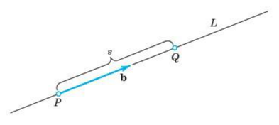
The directional derivative DbfD_{\mathbf{b}}f or df/dsdf/ds of a function f(x,y,z)f(x, y, z) at a point PP in the direction of a vector b\mathbf{b} is defined by Figure 3.10

Dbf=dfds=lim⁡s→0f(Q)−f(P)s.D_{\mathbf{b}}f = \frac{df}{ds} = \lim_{s \to 0}\frac{f(Q) - f(P)}{s}.

Here QQ is a variable point on the straight line LL in the direction of b\mathbf{b}, and ∣s∣|s| is the distance between PP and QQ. Also, s>0s > 0 if QQ lies in the direction of b\mathbf{b} (as in Fig. 3.10), s<0s < 0 if QQ lies in the direction of −b-\mathbf{b}, and s=0s = 0 if Q=PQ = P.

Fig. 3.10 Directional Derivative (Refer to above Equation)

Fig. 3.10 Directional Derivative (Refer to above Equation)

The above equation can be derived into

(dfds)b,P=[(∂f∂x)Pi+(∂f∂y)Pj]⏟Gradient of f at P⋅[b1i+b2j]⏟Direction b\left(\frac{df}{ds}\right)_{\mathbf{b}, P} = \underbrace{\left[\left(\frac{\partial f}{\partial x}\right)_P \mathbf{i} + \left(\frac{\partial f}{\partial y}\right)_P \mathbf{j}\right]}_{\text{Gradient of } f \text{ at } P} \cdot \underbrace{[b_1\mathbf{i} + b_2\mathbf{j}]}_{\text{Direction } \mathbf{b}}

DEFINITION

The gradient vector (gradient) of f(x,y)f(x, y) at a point P0(x0,y0)P_0(x_0, y_0) is the vector

∇f=∂f∂xi+∂f∂yj\nabla f = \frac{\partial f}{\partial x}\mathbf{i} + \frac{\partial f}{\partial y}\mathbf{j}

obtained by evaluating the partial derivatives of ff at P0P_0.

The notation ∇f\nabla f is read "grad ƒ" as well as "gradient of ƒ" and "del ƒ." The symbol ∇\nabla by itself is read "del." Another notation for the gradient is grad ƒ.

The Directional Derivative Is a Dot Product

If f(x,y)f(x, y) is differentiable in an open region containing P(x,y)P(x, y), then

(dfds)b,P=(∇f)P⋅b\left(\frac{df}{ds}\right)_{\mathbf{b}, P} = (\nabla f)_P \cdot \mathbf{b}

the dot product of the gradient ∇f\nabla f at PP and b\mathbf{b}

Example 3.6​

Find the directional derivative of f(x,y,z)=2x2+3y2+z2f(x, y, z) = 2x^2 + 3y^2 + z^2 at PP: (2,1,3)(2, 1, 3) in the direction of a=[1,0,−2]\mathbf{a} = [1, 0, -2].

Solution

grad⁡f=[4x,6y,2z]\operatorname{grad} f = [4x, 6y, 2z] gives at PP the vector grad⁡f(P)=[8,6,6]\operatorname{grad} f(P) = [8, 6, 6]. From this we obtain, since ∣a∣=5|\mathbf{a}| = \sqrt{5},

Daf(P)=15[1,0,−2]⋅[8,6,6]=15(8+0−12)=−45=−1.789.D_{\mathbf{a}}f(P) = \frac{1}{\sqrt{5}}[1, 0, -2] \cdot [8, 6, 6] = \frac{1}{\sqrt{5}}(8 + 0 - 12) = -\frac{4}{\sqrt{5}} = -1.789.

The minus sign indicates that at PP the function ff is decreasing in the direction of a\mathbf{a}.

Example 3.7​

Find the derivative of f(x,y)=xey+cos⁡(xy)f(x, y) = xe^y + \cos(xy) at the point (2,0)(2, 0) in the direction of v=3i−4j\mathbf{v} = 3\mathbf{i} - 4\mathbf{j}.

Solution

The direction of v\mathbf{v} is the unit vector obtained by dividing v\mathbf{v} by its length:

u=v∣v∣=v5=35i−45j.\mathbf{u} = \frac{\mathbf{v}}{|\mathbf{v}|} = \frac{\mathbf{v}}{5} = \frac{3}{5}\mathbf{i} - \frac{4}{5}\mathbf{j}.

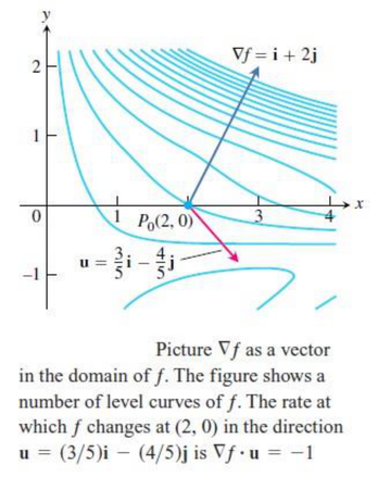
Level curves of f with the gradient vector and the direction u

Picture ∇f as a vector in the domain of f. The figure shows a number of level curves of f. The rate at which f changes at (2, 0) in the direction u = (3/5)i − (4/5)j is ∇f · u = −1

Exercises​

Find the derivative of the function at PoP_o in the direction of uu

(a) g(x,y)=x−yxy+2g(x, y) = \dfrac{x-y}{xy+2}, Po(1,−1)P_o(1, -1), u=12i+5ju = 12\mathbf{i} + 5\mathbf{j}

(b) h(x,y,z)=cos⁡xy+eyz+ln⁡(zx)h(x, y, z) = \cos xy + e^{yz} + \ln(zx), Po(1,0,1/2)P_o(1, 0, 1/2), u=1i+2j+2ku = 1\mathbf{i} + 2\mathbf{j} + 2\mathbf{k}

(c) h(x,y,z)=3excos⁡yzh(x, y, z) = 3e^x\cos yz, Po(0,0,0)P_o(0, 0, 0), u=2i+j−2ku = 2\mathbf{i} + \mathbf{j} - 2\mathbf{k}

3.4.3 Divergence of Vector Field​

From a scalar field we can obtain a vector field by the gradient. Conversely, from a vector field we can obtain a scalar field by the divergence or another vector field by the curl.

To begin, let v(x,y,z)v(x, y, z) be a differentiable vector function, where xx, yy, zz are Cartesian coordinates, and let v1v_1, v2v_2, v3v_3 be the components of v\mathbf{v}. Then the function

div⁡v=∂v1∂x+∂v2∂y+∂v3∂z\operatorname{div} v = \frac{\partial v_1}{\partial x} + \frac{\partial v_2}{\partial y} + \frac{\partial v_3}{\partial z}

is called the divergence of v\mathbf{v} or the divergence of the vector field defined by v\mathbf{v}. For example, if

v=[3xz,2xy,−yz2]=3xz i+2xy j−yz2 kv = [3xz, 2xy, -yz^2] = 3xz\,\mathbf{i} + 2xy\,\mathbf{j} - yz^2\,\mathbf{k}

Then

div⁡v=3z+2x−2yz\operatorname{div} v = 3z + 2x - 2yz

Another common notation for the divergence is

div⁡v=∇⋅v=[∂∂x,∂∂y,∂∂z]⋅[v1,v2,v3]=(∂∂xi+∂∂yj+∂∂zk)⋅[v1i+v2j+v3k]=∂v1∂x+∂v2∂y+∂v3∂z\begin{aligned} \operatorname{div} v = \nabla \cdot v &= \left[\frac{\partial}{\partial x}, \frac{\partial}{\partial y}, \frac{\partial}{\partial z}\right] \cdot [v_1, v_2, v_3] \\ &= \left(\frac{\partial}{\partial x}\mathbf{i} + \frac{\partial}{\partial y}\mathbf{j} + \frac{\partial}{\partial z}\mathbf{k}\right) \cdot [v_1\mathbf{i} + v_2\mathbf{j} + v_3\mathbf{k}] \\ &= \frac{\partial v_1}{\partial x} + \frac{\partial v_2}{\partial y} + \frac{\partial v_3}{\partial z} \end{aligned}

With understanding that the "product" (∂∂x)v1\left(\dfrac{\partial}{\partial x}\right)v_1 in the dot product means the partial derivative ∂v1∂x\dfrac{\partial v_1}{\partial x}, etc. This is a convenient notation, but nothing more. Note that ∇.v\boldsymbol{\nabla}.\boldsymbol{v} means the scalar div v\mathbf{v}, whereas ∇f\boldsymbol{\nabla}f means the vector grad ff.

Example 3.8​

If f(x,y,z)=xz i+xyz j−y2 kf(x, y, z) = xz\,\mathbf{i} + xyz\,\mathbf{j} - y^2\,\mathbf{k}, find div⁡f\operatorname{div} f

Solution
div⁡f=∇⋅f=∂∂x(xz)+∂∂y(xyz)+∂∂z(−y2)=z+xz\begin{aligned} \operatorname{div} f &= \nabla \cdot f \\ &= \frac{\partial}{\partial x}(xz) + \frac{\partial}{\partial y}(xyz) + \frac{\partial}{\partial z}(-y^2) \\ &= z + xz \end{aligned}

*Div F is a scalar field.

Let us turn to the more immediate practical task of gaining a feel for the significance of the divergence. Let f(x,y,z)f(x, y, z) be a twice differentiable scalar function. Then, its gradient exists

v=grad⁡f=[∂f∂x,∂f∂y,∂f∂z]=∂f∂xi+∂f∂yj+∂f∂zkv = \operatorname{grad} f = \left[\frac{\partial f}{\partial x}, \frac{\partial f}{\partial y}, \frac{\partial f}{\partial z}\right] = \frac{\partial f}{\partial x}\mathbf{i} + \frac{\partial f}{\partial y}\mathbf{j} + \frac{\partial f}{\partial z}\mathbf{k}

and we can differentiate once more, the first component with respect to xx, the second with respect to yy, the third with respect to zz, and then form the divergence,

div⁡v=div⁡(grad⁡f)=∂2f∂x2+∂2f∂y2+∂2f∂z2.\operatorname{div} v = \operatorname{div}(\operatorname{grad} f) = \frac{\partial^2 f}{\partial x^2} + \frac{\partial^2 f}{\partial y^2} + \frac{\partial^2 f}{\partial z^2}.

Hence, we have the basic result that the divergence of the gradient is the Laplacian

div⁡(grad⁡f)=∇2f.\operatorname{div}(\operatorname{grad} f) = \nabla^2 f.

Exercises​

  1. Find divergence from the gradient, div (grad f)

    (a) f=exyzf = e^{xyz}

    (b) f=z−x2+y2f = z - \sqrt{x^2 + y^2}

  2. Find div v\boldsymbol{div}\ \boldsymbol{v} and its value at PP

    (a) v=x2i+4y2j+9z2kv = x^2\mathbf{i} + 4y^2\mathbf{j} + 9z^2\mathbf{k} at P(−1,0,12)P(-1, 0, \tfrac{1}{2})

    (b) v=cos⁡xyz+sin⁡xyzv = \cos xyz + \sin xyz

3.4.4 Curl of Vector Field​

Let v(x,y,z)=[v1,v2,v3]=v1i+v2j+v3kv(x, y, z) = [v_1, v_2, v_3] = v_1\mathbf{i} + v_2\mathbf{j} + v_3\mathbf{k} be a differentiable vector function of the Cartesian coordinates xx, yy, zz. Then the curl of the vector function v or of the vector field given by v\mathbf{v} is defined by the "symbolic" determinant

curl⁡v=∇×v=∣ijk∂∂x∂∂y∂∂zv1v2v3∣\operatorname{curl} v = \nabla \times v = \begin{vmatrix} \mathbf{i} & \mathbf{j} & \mathbf{k} \\ \dfrac{\partial}{\partial x} & \dfrac{\partial}{\partial y} & \dfrac{\partial}{\partial z} \\ v_1 & v_2 & v_3 \end{vmatrix}

=(∂v3∂y−∂v2∂z)i+(∂v1∂z−∂v3∂x)j+(∂v2∂x−∂v1∂y)k= \left(\frac{\partial v_3}{\partial y} - \frac{\partial v_2}{\partial z}\right)\mathbf{i} + \left(\frac{\partial v_1}{\partial z} - \frac{\partial v_3}{\partial x}\right)\mathbf{j} + \left(\frac{\partial v_2}{\partial x} - \frac{\partial v_1}{\partial y}\right)\mathbf{k}

This is the formula when xx, yy, zz are right-handed. If they are left-handed, the determinant has a minus sign in front. Instead of curl v\mathbf{v} one also uses the notation rot v\mathbf{v} or rotation of v\mathbf{v}.

Example 3.9​

Let v=[yz,3zx,z]=yz i+3zx j+z k\mathbf{v} = [yz, 3zx, z] = yz\,\mathbf{i} + 3zx\,\mathbf{j} + z\,\mathbf{k} with right-handed xx, yy, zz.

Solution

curl⁡v=∣ijk∂∂x∂∂y∂∂zyz3zxz∣=−3x i+y j+(3z−z)k=−3x i+y j+2z k.\operatorname{curl} \mathbf{v} = \begin{vmatrix} \mathbf{i} & \mathbf{j} & \mathbf{k} \\ \dfrac{\partial}{\partial x} & \dfrac{\partial}{\partial y} & \dfrac{\partial}{\partial z} \\ yz & 3zx & z \end{vmatrix} = -3x\,\mathbf{i} + y\,\mathbf{j} + (3z - z)\mathbf{k} = -3x\,\mathbf{i} + y\,\mathbf{j} + 2z\,\mathbf{k}.

Example 3.10​

If F(x,y,z)=xz i+xyz j−y2 kF(x, y, z) = xz\,\mathbf{i} + xyz\,\mathbf{j} - y^2\,\mathbf{k}, find curl FF

Solution

curl⁡F=∇×F=∣ijk∂∂x∂∂y∂∂zxzxyz−y2∣\operatorname{curl} F = \nabla \times F = \begin{vmatrix} \mathbf{i} & \mathbf{j} & \mathbf{k} \\ \dfrac{\partial}{\partial x} & \dfrac{\partial}{\partial y} & \dfrac{\partial}{\partial z} \\ xz & xyz & -y^2 \end{vmatrix}

=[∂∂y(−y2)−∂∂z(xyz)]i−[∂∂x(−y2)−∂∂z(xz)]j+[∂∂x(xyz)−∂∂y(xz)]k=(−2y−xy)i−(0−x)j+(yz−0)k=−y(2+x) i+x j+yz k\begin{aligned} &= \left[\frac{\partial}{\partial y}(-y^2) - \frac{\partial}{\partial z}(xyz)\right]\mathbf{i} - \left[\frac{\partial}{\partial x}(-y^2) - \frac{\partial}{\partial z}(xz)\right]\mathbf{j} \\ &\quad + \left[\frac{\partial}{\partial x}(xyz) - \frac{\partial}{\partial y}(xz)\right]\mathbf{k} \\ &= (-2y - xy)\mathbf{i} - (0 - x)\mathbf{j} + (yz - 0)\mathbf{k} \\ &= -y(2 + x)\,\mathbf{i} + x\,\mathbf{j} + yz\,\mathbf{k} \end{aligned}

*Curl F is a vector field.

Grad, Div, Curl

Gradient fields are irrotational. That is, if a continuously differentiable vector function is the gradient of a scalar function f, then its curl is the zero vector,

curl⁡(grad⁡f)=0.\operatorname{curl}(\operatorname{grad} f) = \mathbf{0}.

Furthermore, the divergence of the curl of a twice continuously differentiable vector function v\mathbf{v} is zero,

div⁡(curl⁡v)=0.\operatorname{div}(\operatorname{curl} \mathbf{v}) = \mathbf{0}.

Exercises​

Compute the curl of the following vector field:

a) f(x,y,z)=⟨excos⁡y,exsin⁡y,0⟩f(x, y, z) = \langle e^x\cos y, e^x\sin y, 0 \rangle

b) f(x,y,z)=2xyzi+xexyj+cos⁡(xy2)kf(x, y, z) = \dfrac{2xy}{z}\mathbf{i} + xe^{xy}\mathbf{j} + \cos(xy^2)\mathbf{k}

c) f(x,y,z)=(xyz)i+(x2+2yz)j+(x2+y2+z2)kf(x, y, z) = (xyz)\mathbf{i} + (x^2 + 2yz)\mathbf{j} + (x^2 + y^2 + z^2)\mathbf{k}