Lecture 5: Engineering Applications of Vector Algebra and Vector Analysis

Download the original PDF →


5.1 Engineering Application: Vector Algebra​

5.1.1 Head to Tail Method​

Example 5.1​

  1. A 200 kg cylinder is hung by means of two cables ABAB and ACAC, which are attached to the top of a vertical wall. A horizontal force P\mathbf{P} perpendicular to the wall holds the cylinder in the position shown below.
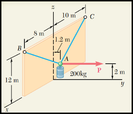
A 200 kg cylinder hung by two cables AB and AC from a vertical wall, held by a horizontal force P

(i) Find the coordinate of position AA, BB and CC and their position vectors based on the axis given in the diagram above.

(ii) Identify all the force vectors acting on point AA. (Assume g=9.81 m s−2g = 9.81\text{ m s}^{-2})

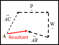
(iii) Determine the resultant of forces acting on point AA using head to-tail method.

(iv) Assume the system is in static, determine the magnitude of P\mathbf{P} and the tension in each cable.

Solution

In this example, you should be able to solve 3D engineering problem using vector. Hint: imagine 3D object and translate it in the point point (i.e. A=(1,2,3)A = (1,2,3)), B=(2,3,4)B = (2,3,4) and vector form (i.e. position vector OA→=⟨1,2,3⟩\overrightarrow{OA} = \langle 1,2,3\rangle, OA→=⟨2,3,4⟩\overrightarrow{OA} = \langle 2,3,4\rangle and arbitrary vector AB→=⟨1,1,1⟩\overrightarrow{AB} = \langle 1,1,1\rangle, BA→=⟨−1,−1,−1⟩\overrightarrow{BA} = \langle -1,-1,-1\rangle)

(i) Find the coordinate of position AA, BB and CC and their position vectors based on the axis given in the diagram.

A=(0,1.2,2),B=(8,0,12),C=(−10,0,12)A = (0, 1.2, 2), \qquad B = (8, 0, 12), \qquad C = (-10, 0, 12)

OA→=⟨0,1.2,2⟩,OB→=⟨8,0,12⟩,OC→=⟨−10,0,12⟩\overrightarrow{OA} = \langle 0, 1.2, 2\rangle, \qquad \overrightarrow{OB} = \langle 8, 0, 12\rangle, \qquad \overrightarrow{OC} = \langle -10, 0, 12\rangle

(ii) Identify all the force vectors acting on point AA. (Assume g=9.81 m s−2g = 9.81\text{ m s}^{-2})

Horizontal force P\mathbf{P}, & its vector P=⟨0,P,0⟩\mathbf{P} = \langle 0, P, 0\rangle (note it has magnitude PP in yy direction)

Vertical force 200 kg cylinder, and its vector W=⟨0,0,−1962N⟩\mathbf{W} = \langle 0, 0, -1962N\rangle (note it has magnitude 1962N in negative zz direction)

Tension cable AB, and its vector

TAB=∣TAB∣⏟MagnitudeAB^⏟Direction vector\mathbf{T}_{AB} = \underbrace{\lvert \mathbf{T}_{AB}\rvert}_{\text{Magnitude}} \underbrace{\widehat{AB}}_{\text{Direction vector}}

The magnitude is unknown (Precaution: the magnitude of vector ∣AB→∣\lvert\overrightarrow{AB}\rvert is not equal to the magnitude of tension ∣TAB→∣\lvert\overrightarrow{T_{AB}}\rvert)

The direction vector (unit vector) is the same as the unit vector of AB→\overrightarrow{AB}

AB→=OB→−OA→=⟨8,0,12⟩−⟨0,1.2,2⟩=⟨8,−1.2,10⟩\overrightarrow{AB} = \overrightarrow{OB} - \overrightarrow{OA} = \langle 8, 0, 12\rangle - \langle 0, 1.2, 2\rangle = \langle 8, -1.2, 10\rangle

AB^=⟨8,−1.2,10⟩82+(−1.2)2+102=⟨8,−1.2,10⟩165.44=⟨0.6220,−0.09330,0.7775⟩\widehat{AB} = \frac{\langle 8, -1.2, 10\rangle}{\sqrt{8^2 + (-1.2)^2 + 10^2}} = \frac{\langle 8, -1.2, 10\rangle}{\sqrt{165.44}} = \langle 0.6220, -0.09330, 0.7775\rangle

TAB=∣TAB∣⏟MagnitudeTAB^⏟Direction vector=∣TAB∣AB^=∣TAB∣⟨0.6220,−0.09330,0.7775⟩\mathbf{T}_{AB} = \underbrace{\lvert \mathbf{T}_{AB}\rvert}_{\text{Magnitude}} \underbrace{\widehat{T_{AB}}}_{\text{Direction vector}} = \lvert \mathbf{T}_{AB}\rvert \widehat{AB} = \lvert \mathbf{T}_{AB}\rvert \langle 0.6220, -0.09330, 0.7775\rangle

Tension cable AC, & its vector TAC=∣TAC∣⏟MagnitudeTAC^⏟Direction vector\mathbf{T}_{AC} = \underbrace{\lvert \mathbf{T}_{AC}\rvert}_{\text{Magnitude}} \underbrace{\widehat{T_{AC}}}_{\text{Direction vector}}

AC→=OC→−OA→=⟨−10,0,12⟩−⟨0,1.2,2⟩=⟨−10,−1.2,10⟩\overrightarrow{AC} = \overrightarrow{OC} - \overrightarrow{OA} = \langle -10, 0, 12\rangle - \langle 0, 1.2, 2\rangle = \langle -10, -1.2, 10\rangle

AC^=⟨−10,−1.2,10⟩(−10)2+(−1.2)2+102=⟨−10,−1.2,10⟩201.44=⟨−0.7046,−0.08455,0.7046⟩\widehat{AC} = \frac{\langle -10, -1.2, 10\rangle}{\sqrt{(-10)^2 + (-1.2)^2 + 10^2}} = \frac{\langle -10, -1.2, 10\rangle}{\sqrt{201.44}} = \langle -0.7046, -0.08455, 0.7046\rangle

TAC=∣TAC∣⏟MagnitudeTAC^⏟Direction vector=∣TAC∣AC^=∣TAC∣⟨−0.7046,−0.08455,0.7046⟩\mathbf{T}_{AC} = \underbrace{\lvert \mathbf{T}_{AC}\rvert}_{\text{Magnitude}} \underbrace{\widehat{T_{AC}}}_{\text{Direction vector}} = \lvert \mathbf{T}_{AC}\rvert \widehat{AC} = \lvert \mathbf{T}_{AC}\rvert \langle -0.7046, -0.08455, 0.7046\rangle

(iii) Determine the resultant of forces acting on point AA using head to-tail method.

The forces AB, AC, P and W drawn head to tail at point A

The resultant polygon of AB, AC, P and W, with the resultant drawn from A

The resultant of force is the addition of vectors AB→\overrightarrow{AB}, AC→\overrightarrow{AC}, P\mathbf{P}, and W\mathbf{W} where

Resultant, ΣF\Sigma F

=∣TAC∣⟨−0.7046,−0.08455,0.7046⟩+∣TAB∣⟨0.6220,−0.09330,0.7775⟩+⟨0,P,0⟩+⟨0,0,−1962N⟩=⟨{−0.7046∣TAC∣+0.6220∣TAB∣},{−0.08455∣TAC∣−0.09330∣TAB∣+P},{0.7046∣TAC∣+0.7775∣TAB∣−1962N}⟩\begin{aligned} &= \lvert \mathbf{T}_{AC}\rvert \langle -0.7046, -0.08455, 0.7046\rangle + \lvert \mathbf{T}_{AB}\rvert \langle 0.6220, -0.09330, 0.7775\rangle + \langle 0, P, 0\rangle + \langle 0, 0, -1962N\rangle \\ &= \langle \{-0.7046\lvert \mathbf{T}_{AC}\rvert + 0.6220\lvert \mathbf{T}_{AB}\rvert\}, \{-0.08455\lvert \mathbf{T}_{AC}\rvert - 0.09330\lvert \mathbf{T}_{AB}\rvert + P\}, \{0.7046\lvert \mathbf{T}_{AC}\rvert + 0.7775\lvert \mathbf{T}_{AB}\rvert - 1962N\}\rangle \end{aligned}

(iv) Assume the system is in static, determine the magnitude of PP and the tension in each cable.

Since the object is in equilibrium, hence the resultant of force at point AA must be equal to zero, ΣF=0\Sigma F = 0

⟨{−0.7046∣TAC∣+0.6220∣TAB∣},{−0.08455∣TAC∣−0.09330∣TAB∣+P},{0.7046∣TAC∣+0.7775∣TAB∣−1962N}⟩=0\langle \{-0.7046\lvert \mathbf{T}_{AC}\rvert + 0.6220\lvert \mathbf{T}_{AB}\rvert\}, \{-0.08455\lvert \mathbf{T}_{AC}\rvert - 0.09330\lvert \mathbf{T}_{AB}\rvert + P\}, \{0.7046\lvert \mathbf{T}_{AC}\rvert + 0.7775\lvert \mathbf{T}_{AB}\rvert - 1962N\}\rangle = 0

ΣFx=0\Sigma F_x = 0

{−0.7046∣TAC∣+0.6220∣TAB∣}=0  ⟹  ∣TAC∣=0.62200.7046∣TAB∣\{-0.7046\lvert \mathbf{T}_{AC}\rvert + 0.6220\lvert \mathbf{T}_{AB}\rvert\} = 0 \implies \lvert \mathbf{T}_{AC}\rvert = \frac{0.6220}{0.7046}\lvert \mathbf{T}_{AB}\rvert

ΣFz=0\Sigma F_z = 0

0.7046(0.62200.7046∣TAB∣)+0.7775∣TAB∣−1962N=0  ⟹  ∣TAB∣=1401.93N0.7046\left(\frac{0.6220}{0.7046}\lvert \mathbf{T}_{AB}\rvert\right) + 0.7775\lvert \mathbf{T}_{AB}\rvert - 1962N = 0 \implies \lvert \mathbf{T}_{AB}\rvert = 1401.93N

∣TAC∣=0.62200.7046(1401.93)=1237.58N\lvert \mathbf{T}_{AC}\rvert = \frac{0.6220}{0.7046}(1401.93) = 1237.58N

ΣFy=0\Sigma F_y = 0

−0.08455∣TAC∣−0.09330∣TAB∣+P=0  ⟹  -0.08455\lvert \mathbf{T}_{AC}\rvert - 0.09330\lvert \mathbf{T}_{AB}\rvert + P = 0 \implies

P=235.44NP = 235.44N

5.1.2 Engineering Application: Vector in 3 D Space​

Example 5.2​

The wire AE, L1L_1 is stretched between the corners A and E of a bent plate. The wire BF, L2L_2 is stretched between the position B and F. The wire BG, L3L_3 is stretched between the position B and G. The wire OA, L4L_4 is stretched between the position O and A.
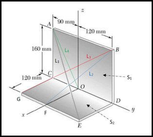
A bent plate in 3D space with the wires L1, L2, L3 and L4 and the planes S1 and S2

(i) Find the vector equation of line for wire AE, BF, BG and OA. Hence find the intersection point between line L1L_1 with L2L_2; line L3L_3 with L4L_4 separately if exist.

(ii) Find the equation of plane for S1S_1 from point O, A & B and equation of plane for S2S_2 from point E, F and G if possible. Hence find the intersection line between S1S_1 and S2S_2 if exist.

(iii) Given the intersection point between L1L_1 & L3L_3 is P(60,15,80)P(60, 15, 80). Find the shortest distance between intersection point L1L_1 & L3L_3 and plane S1S_1 and plane S2S_2 respectively.

Solution

(i)

Vector equation of line for wire BF

Point B=(0,120,160)B = (0,120,160) and F=(120,0,0)F = (120,0,0)

Position vector, OB→=⟨0,120,160⟩\overrightarrow{OB} = \langle 0,120,160\rangle, OF→=⟨120,0,0⟩\overrightarrow{OF} = \langle 120,0,0\rangle

Vector BF→=OF→−OB→=⟨120,0,0⟩−⟨0,120,160⟩=⟨120,−120,−160⟩\overrightarrow{BF} = \overrightarrow{OF} - \overrightarrow{OB} = \langle 120,0,0\rangle - \langle 0,120,160\rangle = \langle 120,-120,-160\rangle

L2=OB→+tBF→=⟨0,120,160⟩+t⟨120,−120,−160⟩L_2 = \overrightarrow{OB} + t\overrightarrow{BF} = \langle 0,120,160\rangle + t\langle 120,-120,-160\rangle

Vector equation of line for wire BG

Point B=(0,120,160)B = (0,120,160) and G=(120,−90,0)G = (120,-90,0)

Position vector, OB→=⟨0,120,160⟩\overrightarrow{OB} = \langle 0,120,160\rangle, OG→=⟨120,−90,0⟩\overrightarrow{OG} = \langle 120,-90,0\rangle

Vector BG→=OG→−OB→=⟨120,−90,0⟩−⟨0,120,160⟩=⟨120,−210,−160⟩\overrightarrow{BG} = \overrightarrow{OG} - \overrightarrow{OB} = \langle 120,-90,0\rangle - \langle 0,120,160\rangle = \langle 120,-210,-160\rangle

L3=OB→+uBG→=⟨0,120,160⟩+u⟨120,−210,−160⟩L_3 = \overrightarrow{OB} + u\overrightarrow{BG} = \langle 0,120,160\rangle + u\langle 120,-210,-160\rangle

Vector equation of line for wire AE

Point A=(0,−90,160)A = (0,-90,160) and E=(120,120,0)E = (120,120,0)

Position vector, OA→=⟨0,−90,160⟩\overrightarrow{OA} = \langle 0,-90,160\rangle, OE→=⟨120,120,0⟩\overrightarrow{OE} = \langle 120,120,0\rangle

Vector AE→=OE→−OA→=⟨120,120,0⟩−⟨0,−90,160⟩=⟨120,210,−160⟩\overrightarrow{AE} = \overrightarrow{OE} - \overrightarrow{OA} = \langle 120,120,0\rangle - \langle 0,-90,160\rangle = \langle 120,210,-160\rangle

L1=OA→+sAE→=⟨0,−90,160⟩+s⟨120,210,−160⟩L_1 = \overrightarrow{OA} + s\overrightarrow{AE} = \langle 0,-90,160\rangle + s\langle 120,210,-160\rangle

Vector equation of line for wire OA

Point O=(0,0,0)O = (0,0,0) and A=(0,−90,160)A = (0,-90,160)

Position vector, OO→=⟨0,0,0⟩\overrightarrow{OO} = \langle 0,0,0\rangle, OA→=⟨0,−90,160⟩\overrightarrow{OA} = \langle 0,-90,160\rangle

Vector OA→=OA→−OO→=⟨0,−90,160⟩−⟨0,0,0⟩=⟨0,−90,160⟩\overrightarrow{OA} = \overrightarrow{OA} - \overrightarrow{OO} = \langle 0,-90,160\rangle - \langle 0,0,0\rangle = \langle 0,-90,160\rangle

L4=OO→+vOA→=⟨0,0,0⟩+v⟨0,−90,160⟩=v⟨0,−90,160⟩L_4 = \overrightarrow{OO} + v\overrightarrow{OA} = \langle 0,0,0\rangle + v\langle 0,-90,160\rangle = v\langle 0,-90,160\rangle

To check existence of intersection point between L1 & L2:

L1=OA→+sAE→=⟨0,−90,160⟩+s⟨120,210,−160⟩L_1 = \overrightarrow{OA} + s\overrightarrow{AE} = \langle 0,-90,160\rangle + s\langle 120,210,-160\rangle

L2=OB→+tBF→=⟨0,120,160⟩+t⟨120,−120,−160⟩L_2 = \overrightarrow{OB} + t\overrightarrow{BF} = \langle 0,120,160\rangle + t\langle 120,-120,-160\rangle

L1=L2L_1 = L_2

⟨0,−90,160⟩+s⟨120,210,−160⟩=⟨0,120,160⟩+t⟨120,−120,−160⟩\langle 0,-90,160\rangle + s\langle 120,210,-160\rangle = \langle 0,120,160\rangle + t\langle 120,-120,-160\rangle

120s=120t  ⟹  s=t— (1)120s = 120t \implies s = t \qquad \text{--- (1)}

160−160s=160−160t  ⟹  s=t— (2)160 - 160s = 160 - 160t \implies s = t \qquad \text{--- (2)}

−90+210s=120−120t  ⟹  −210−330=t— (3)-90 + 210s = 120 - 120t \implies \frac{-210}{-330} = t \qquad \text{--- (3)}

LHS:−90+210(−210−330)=43.6364LHS: -90 + 210\left(\frac{-210}{-330}\right) = 43.6364

RHS:120−120(−210−330)=43.6364RHS: 120 - 120\left(\frac{-210}{-330}\right) = 43.6364

LHS=RHSLHS = RHS

There is intersection point between L1 & L2.

L1=L2L_1 = L_2

=⟨0,−90,160⟩+210330⟨120,210,−160⟩=⟨0,120,160⟩+210330⟨120,−120,−160⟩=⟨76.363643.636458.1818⟩\begin{aligned} &= \langle 0,-90,160\rangle + \frac{210}{330}\langle 120,210,-160\rangle \\ &= \langle 0,120,160\rangle + \frac{210}{330}\langle 120,-120,-160\rangle \\ &= \langle 76.3636 \quad 43.6364 \quad 58.1818\rangle \end{aligned}

The intersection point is at (76.3636,43.6364,58.1818)(76.3636, 43.6364, 58.1818)

To check existence of intersection point between L3 & L4:

L3=OB→+uBG→=⟨0,120,160⟩+u⟨120,−210,−160⟩L_3 = \overrightarrow{OB} + u\overrightarrow{BG} = \langle 0,120,160\rangle + u\langle 120,-210,-160\rangle

L4=OO→+vOA→=⟨0,0,0⟩+v⟨0,−90,160⟩=v⟨0,−90,160⟩L_4 = \overrightarrow{OO} + v\overrightarrow{OA} = \langle 0,0,0\rangle + v\langle 0,-90,160\rangle = v\langle 0,-90,160\rangle

L3=L4L_3 = L_4

⟨0,120,160⟩+u⟨120,−210,−160⟩=v⟨0,−90,160⟩\langle 0,120,160\rangle + u\langle 120,-210,-160\rangle = v\langle 0,-90,160\rangle

120u=0  ⟹  u=0120u = 0 \implies u = 0

120−210u=−90v  ⟹  v=−43120 - 210u = -90v \implies v = -\frac{4}{3}

160−160u=160v160 - 160u = 160v

LHS:160−160(0)=160LHS: 160 - 160(0) = 160

RHS:160(−43)=−213.33RHS: 160\left(-\frac{4}{3}\right) = -213.33

LHS≠RHSLHS \neq RHS

There is no intersection point between L3 & L4.

(ii)

To form equation of plane for S1S_1, we need three points located on the plane:

Point A=(0,−90,160)A = (0,-90,160)

Point B=(0,120,160)B = (0,120,160)

Point O=(0,0,0)O = (0,0,0)

The format for equation of plane: ax+by+cz=kax + by + cz = k where the normal vector to the plane is ⟨a,b,c⟩\langle a,b,c\rangle

Normal vector to the plane=OA→×OB→=∣i‾j‾k‾0−901600120160∣=⟨−33600,0,0⟩\text{Normal vector to the plane} = \overrightarrow{OA} \times \overrightarrow{OB} = \begin{vmatrix} \underline{i} & \underline{j} & \underline{k} \\ 0 & -90 & 160 \\ 0 & 120 & 160 \end{vmatrix} = \langle -33600, 0, 0\rangle

Hence we get, ax+by+cz=k  ⟹  −33600x+0y+0z=k  ⟹  k=−33600xax + by + cz = k \implies -33600x + 0y + 0z = k \implies k = -33600x

From the point located on S1S_1, i.e., point OO, AA and BB. All the component at xx direction is 0. Sub to the equation we get k=−33600x=0k = -33600x = 0; Thus, the plane of equation is −33600x=0-33600x = 0 which can be simplify to x=0x = 0

Note: normal vector ⟨−33600,0,0⟩\langle -33600, 0, 0\rangle is parallel to ⟨1,0,0⟩\langle 1, 0, 0\rangle

To form equation of plane for S2S_2, we need three points located on the plane:

Point E=(120,120,0)E = (120,120,0)

Point F=(120,0,0)F = (120,0,0)

Point G=(120,−90,0)G = (120,-90,0)

The format for equation of plane: ax+by+cz=kax + by + cz = k where the normal vector to the plane is ⟨a,b,c⟩\langle a,b,c\rangle

Normal vector to the plane=EF→×EG→=∣i‾j‾k‾0−12000−2100∣=⟨0,0,0⟩\text{Normal vector to the plane} = \overrightarrow{EF} \times \overrightarrow{EG} = \begin{vmatrix} \underline{i} & \underline{j} & \underline{k} \\ 0 & -120 & 0 \\ 0 & -210 & 0 \end{vmatrix} = \langle 0, 0, 0\rangle

The normal vector is a zero vector, this result is invalid because the points that we selected to form a plane must be non-collinear. Note that we can't find the normal vector by using cross product of parallel vectors as ∣v1×v2∣=∥v1∥∥v2∥sin⁡θ n=0\lvert v_1 \times v_2\rvert = \lVert v_1\rVert \lVert v_2\rVert \sin\theta\, n = 0. However, in this case, the vector EF→\overrightarrow{EF} and EG→\overrightarrow{EG} are in parallel. Therefore, it is impossible to use the selected points to calculate the plane of equation.

Thus a new point O=(0,0,0)O = (0,0,0) is selected to avoid this issue.

Normal vector to the plane=OE→×OF→=∣i‾j‾k‾120120012000∣=⟨0,0,−14400⟩\text{Normal vector to the plane} = \overrightarrow{OE} \times \overrightarrow{OF} = \begin{vmatrix} \underline{i} & \underline{j} & \underline{k} \\ 120 & 120 & 0 \\ 120 & 0 & 0 \end{vmatrix} = \langle 0, 0, -14400\rangle

Hence we get, ax+by+cz=k  ⟹  0x+0y−14400z=k  ⟹  k=−14400zax + by + cz = k \implies 0x + 0y - 14400z = k \implies k = -14400z

From the point located on S2S_2, i.e., point OO, EE and FF. All the component at zz direction is 0. Sub to the equation we get k=−14400z=0k = -14400z = 0; Thus, the plane of equation is −14400z=0-14400z = 0 which can be simplify to z=0z = 0

Note: normal vector ⟨0,0,−14400⟩\langle 0, 0, -14400\rangle is parallel to ⟨0,0,1⟩\langle 0, 0, 1\rangle

(iii)

Equation of plane for S1S_1 is x=0x=0 while S2S_2 is z=0z=0. The normal vector to plane S1S_1 is ⟨1,0,0⟩\langle 1, 0, 0\rangle and normal vector to plane S2S_2 is ⟨0,0,1⟩\langle 0, 0, 1\rangle

Thus, the arbitrary point at plane S2S_2 is (x y 0)(x\ y\ 0) while arbitrary point at plane S1S_1 is (0 y z)(0\ y\ z)

Let point M=(1 1 0)M = (1\ 1\ 0) located on plane S2S_2 while point N=(0 1 1)N = (0\ 1\ 1) located on plane S1S_1

MP→=OP→−OM→=⟨60 15 80⟩−⟨1 1 0⟩=⟨59 14 80⟩\overrightarrow{MP} = \overrightarrow{OP} - \overrightarrow{OM} = \langle 60\ 15\ 80\rangle - \langle 1\ 1\ 0\rangle = \langle 59\ 14\ 80\rangle

Shortest distance between intersection point L1L_1 & L3L_3 and plane S2S_2 is

∣MP→⋅⟨0 0 1⟩∣=∣⟨59 14 80⟩⋅⟨0 0 1⟩∣=80 unit\lvert \overrightarrow{MP} \cdot \langle 0\ 0\ 1\rangle\rvert = \lvert \langle 59\ 14\ 80\rangle \cdot \langle 0\ 0\ 1\rangle\rvert = 80\ \text{unit}

NP→=OP→−ON→=⟨60 15 80⟩−⟨0 1 1⟩=⟨60 14 79⟩\overrightarrow{NP} = \overrightarrow{OP} - \overrightarrow{ON} = \langle 60\ 15\ 80\rangle - \langle 0\ 1\ 1\rangle = \langle 60\ 14\ 79\rangle

Shortest distance between intersection point L1L_1 & L3L_3 and plane S1S_1 is

∣NP→⋅⟨1 0 0⟩∣=∣⟨60 14 79⟩⋅⟨1 0 0⟩∣=60 unit\lvert \overrightarrow{NP} \cdot \langle 1\ 0\ 0\rangle\rvert = \lvert \langle 60\ 14\ 79\rangle \cdot \langle 1\ 0\ 0\rangle\rvert = 60\ \text{unit}


5.2 Engineering Application: Vector Analysis​

5.2.1 Navigation​

The word problems encountered most often with vectors are navigation problems. These navigation problems use variables like speed and direction to form vectors for computation. Some navigation problems ask us to find the groundspeed of an aircraft using the combined forces of the wind and the aircraft. For these problems it is important to understand the resultant of two forces and the components of force.

Each of the three vectors in the triangle of velocities has two properties: magnitude and direction. This means that there are a total of six components. These are the True Air Speed (TAS) and heading (HDG) of the aircraft, the speed and direction of the wind (W/V), and the Ground Speed (GS) and track (TR) of the path over the ground. This is shown in Figure 5.1.
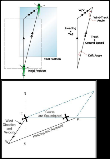
Figure 5.1: Triangle of Vectors (Velocities)

Figure 5.1: Triangle of Vectors (Velocities)

To summarize:

Course—the direction of a line drawn on a chart representing the intended airplane path, expressed as the angle measured from a specific reference datum clockwise from 0° through 360° to the line.

Heading—is the direction in which the nose of the airplane points during flight.

Drift angle—is the angle between heading and track.

Airspeed—is the rate of the airplane's progress through the air.

Groundspeed—is the rate of the airplane's in-flight progress over the ground.

Example 5.3​

A jet airliner, flying due east at 500 mph in still air, encounters a 70-mph tailwind blowing in the direction 60° north of east. The airplane holds its compass heading due east but, because of the wind, acquires a new ground speed and direction. What are they?
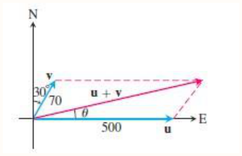
The vectors u (500 due east), v (70 at 30° to the north axis) and the resultant u + v with drift angle theta

Solution

If u=\mathbf{u} = the velocity of the airplane alone and v=\mathbf{v} = the velocity of the tailwind, then ∣u∣=500\lvert\mathbf{u}\rvert = 500 and ∣v∣=70\lvert\mathbf{v}\rvert = 70 (figure above). The velocity of the airplane with respect to the ground is given by the magnitude and direction of the resultant vector u+v\mathbf{u} + \mathbf{v}. If we let the positive xx-axis represent east and the positive yy-axis represent north, then the component forms of u\mathbf{u} and v\mathbf{v} are

u=⟨500,0⟩andv=⟨70cos⁡60∘,70sin⁡60∘⟩=⟨35,353⟩.\mathbf{u} = \langle 500, 0\rangle \qquad \text{and} \qquad \mathbf{v} = \langle 70\cos 60^\circ, 70\sin 60^\circ\rangle = \langle 35, 35\sqrt{3}\rangle.

Therefore,

u+v=⟨535,353⟩=535i+353j\mathbf{u} + \mathbf{v} = \langle 535, 35\sqrt{3}\rangle = 535\mathbf{i} + 35\sqrt{3}\mathbf{j}

∣u+v∣=5352+(353)2≈538.4\lvert\mathbf{u} + \mathbf{v}\rvert = \sqrt{535^2 + (35\sqrt{3})^2} \approx 538.4

and

θ=tan⁡−1353535≈6.5∘.\theta = \tan^{-1}\frac{35\sqrt{3}}{535} \approx 6.5^\circ.

The new ground speed of the airplane is about 538.4 mph, and its new direction is about 6.5° north of east.

Example 5.4​

A 75 N weight is suspended by two wires as shown in figure above. Find the forces F1 and F2 acting in both wires.
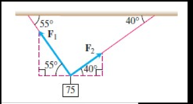
A 75 N weight suspended by two wires making 55 degrees and 40 degrees with the horizontal, with F1 and F2 shown

Solution

The force vectors F1\mathbf{F}_1 and F2\mathbf{F}_2 have magnitudes ∣F1∣\lvert\mathbf{F}_1\rvert and ∣F2∣\lvert\mathbf{F}_2\rvert and components that are measured in Newtons. The resultant force is the sum F1+F2\mathbf{F}_1 + \mathbf{F}_2 and must be equal in magnitude and acting in the opposite (or upward) direction to the weight vector w\mathbf{w}
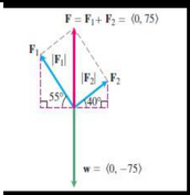
The force triangle for Example 5.4: F = F1 + F2 = (0, 75) and w = (0, -75)

F1=⟨−∣F1∣cos⁡55∘,∣F1∣sin⁡55∘⟩andF2=⟨∣F2∣cos⁡40∘,∣F2∣sin⁡40∘⟩.\mathbf{F}_1 = \langle -\lvert\mathbf{F}_1\rvert\cos 55^\circ, \lvert\mathbf{F}_1\rvert\sin 55^\circ\rangle \qquad \text{and} \qquad \mathbf{F}_2 = \langle \lvert\mathbf{F}_2\rvert\cos 40^\circ, \lvert\mathbf{F}_2\rvert\sin 40^\circ\rangle.

Since F1+F2=⟨0,75⟩\mathbf{F}_1 + \mathbf{F}_2 = \langle 0, 75\rangle, the resultant vector leads to the system of equations

−∣F1∣cos⁡55∘+∣F2∣cos⁡40∘=0-\lvert\mathbf{F}_1\rvert\cos 55^\circ + \lvert\mathbf{F}_2\rvert\cos 40^\circ = 0

∣F1∣sin⁡55∘+∣F2∣sin⁡40∘=75.\lvert\mathbf{F}_1\rvert\sin 55^\circ + \lvert\mathbf{F}_2\rvert\sin 40^\circ = 75.

Solving for ∣F2∣\lvert\mathbf{F}_2\rvert in the first equation and substituting the result into the second equation, we get

∣F2∣=∣F1∣cos⁡55∘cos⁡40∘and∣F1∣sin⁡55∘+∣F1∣cos⁡55∘cos⁡40∘sin⁡40∘=75.\lvert\mathbf{F}_2\rvert = \frac{\lvert\mathbf{F}_1\rvert\cos 55^\circ}{\cos 40^\circ} \qquad \text{and} \qquad \lvert\mathbf{F}_1\rvert\sin 55^\circ + \frac{\lvert\mathbf{F}_1\rvert\cos 55^\circ}{\cos 40^\circ}\sin 40^\circ = 75.

It follows that

∣F1∣=75sin⁡55∘+cos⁡55∘tan⁡40∘≈57.67 N,\lvert\mathbf{F}_1\rvert = \frac{75}{\sin 55^\circ + \cos 55^\circ \tan 40^\circ} \approx 57.67\text{ N},

and

∣F2∣=75cos⁡55∘sin⁡55∘cos⁡40∘+cos⁡55∘sin⁡40∘=75cos⁡55∘sin⁡(55∘+40∘)≈43.18 N.\begin{aligned} \lvert\mathbf{F}_2\rvert &= \frac{75\cos 55^\circ}{\sin 55^\circ\cos 40^\circ + \cos 55^\circ\sin 40^\circ} \\ &= \frac{75\cos 55^\circ}{\sin(55^\circ + 40^\circ)} \approx 43.18\text{ N}. \end{aligned}

Exercises​

  1. A boat leaves port on a heading of 40° with the automatic pilot set for 12 knots. On this particular day, there is a 6-knot current with a heading of 75°.

    a. Sketch and label vectors to represent the intended path of the boat, the current and the resultant path of the boat with the effects of the current.

    b. Calculate the speed and heading at which the boat will actually travel due to the effects of the current.

  2. A plane leaves the airport on a heading 45° traveling a 400 mph. The wind is blowing at a heading of 135° at a speed of 40 mph. What is the actual velocity of the plane?

  3. Consider a 100-N weight suspended by two wires as shown in the accompanying figure. Find the magnitudes and components of the force vectors F1 and F2.
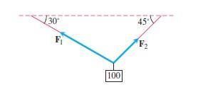
A 100 N weight suspended by two wires, with F1 and F2 shown

5.2.2 Dot Product (Work Done)​

After investigating the dot product, we apply it to finding the projection of one vector onto another (as displayed in Figure 5.2) and to finding the work done by a constant force acting through a displacement.

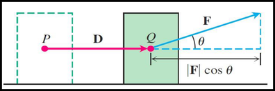
The scalar quantity we seek is the length ∣F∣cos⁡θ\lvert\mathbf{F}\rvert \cos\theta where θ\theta is the angle between the two vectors F\mathbf{F} and D\mathbf{D}. Then

Work=(scalar component of Fin the direction of D)(length of D)=(∣F∣cos⁡θ)∣D∣=F⋅D.\begin{aligned} \text{Work} &= \left(\frac{\text{scalar component of } \mathbf{F}}{\text{in the direction of } \mathbf{D}}\right)(\text{length of } \mathbf{D}) \\ &= (\lvert\mathbf{F}\rvert\cos\theta)\lvert\mathbf{D}\rvert \\ &= \mathbf{F}\cdot\mathbf{D}. \end{aligned}

Figure 5.2: The work done by a constant force F during a displacement D

Figure 5.2: The work done by a constant force F during a displacement D is |F| cos θ, which is the dot product F.D.

Forces Perpendicular to the Motion Do No Work​

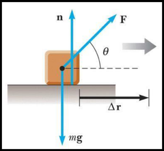
When an object is displaced horizontally on a flat table, the normal force n\mathbf{n} and the gravitational force Fg\mathbf{F}_g do no work since cos⁡90∘=0\cos 90^\circ = 0

A block displaced horizontally on a table by a force F at an angle theta, with the normal force n and the weight mg

Definition

The work done by a constant force F\mathbf{F} acting through a displacement D=PQ→\mathbf{D} = \overrightarrow{PQ} is

W=F⋅D.W = \mathbf{F}\cdot\mathbf{D}.

Example 5.5​

If ∣F∣=40 N\lvert\mathbf{F}\rvert = 40\ N (newtons), D=∣D∣=3 mD = \lvert\mathbf{D}\rvert = 3\ m, and θ=60∘\theta = 60^\circ, the work done by F\mathbf{F} in acting from P to Q is

Solution
Work=F⋅DDefinition=∣F∣∣D∣cos⁡θ=(40)(3)cos⁡60∘Given values=(120)(1/2)=60 J (joules).\begin{aligned} \text{Work} &= \mathbf{F}\cdot\mathbf{D} && \text{Definition} \\ &= \lvert\mathbf{F}\rvert\lvert\mathbf{D}\rvert\cos\theta \\ &= (40)(3)\cos 60^\circ && \text{Given values} \\ &= (120)(1/2) = 60\text{ J (joules)}. \end{aligned}

Exercises​

  1. How much work does it take to slide a crate 20 m along a loading dock by pulling on it with a 200 N force at an angle of 30° from the horizontal?

  2. A 30 kg box is placed 10 m up a ramp that is inclined at 23° to the horizontal. Calculate the work done by the force of gravity as the box slides down to the bottom of the ramp.

5.2.3 Torque (Cross Product)​

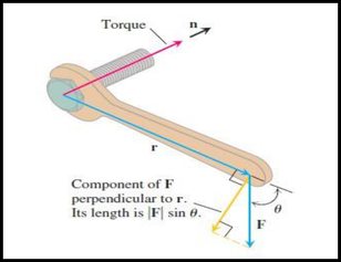
When we turn a bolt by applying a force F to a wrench (Figure 5.3), we produce a torque that causes the bolt to rotate.

The torque vector points in the direction of the axis of the bolt according to the right-hand rule (so the rotation is counter clockwise when viewed from the tip of the vector).

The magnitude of the torque depends on how far out on the wrench the force is applied and on how much of the force is perpendicular to the wrench at the point of application.

The number we use to measure the torque's magnitude is the product of the length of the lever arm rr and the scalar component of FF perpendicular to rr.

Magnitude of torque vector=∣r∣∣F∣sin⁡θ,or∣r×F∣\text{Magnitude of torque vector} = \lvert r\rvert\lvert F\rvert\sin\theta, \qquad \text{or} \qquad \lvert r \times F\rvert

If we let nn be a unit vector along the axis of the bolt in the direction of the torque, then a complete description of the torque vector is
Torque vector=(∣r∣∣F∣sin⁡θ)n,orr×F\text{Torque vector} = (\lvert r\rvert\lvert F\rvert\sin\theta)n, \qquad \text{or} \qquad r \times F

Fig 5.3: The torque vector describes the tendency of the force F to drive the bolt forward

Fig 5.3: The torque vector describes the tendency of the force F to drive the bolt forward.

Example 5.6​

Find the magnitude of the torque generated by force F at the pivot point P in Figure 5.4 is
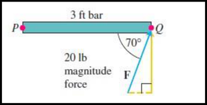
Figure 5.4: Torque exerted by F at P

Figure 5.4: Torque exerted by F at P
Solution
∣PQ→×F∣=∣PQ→∣∣F∣sin⁡70∘≈(3)(20)(0.94)≈56.4 ft-lb.\begin{aligned} \lvert\overrightarrow{PQ} \times \mathbf{F}\rvert &= \lvert\overrightarrow{PQ}\rvert\lvert\mathbf{F}\rvert\sin 70^\circ \\ &\approx (3)(20)(0.94) \\ &\approx 56.4\text{ ft-lb}. \end{aligned}

The magnitude of the torque exerted by F at P is about 56.4 ft-lb. The bar rotates counterclockwise around P.

5.2.4 Triple Scalar or Box Product​

The product is called the triple scalar product of u, v, and w (in that order). As you can see from the formula

∣(u×v)⋅w∣=∣u×v∣∣w∣∣cos⁡θ∣\lvert(\mathbf{u} \times \mathbf{v})\cdot\mathbf{w}\rvert = \lvert\mathbf{u} \times \mathbf{v}\rvert\lvert\mathbf{w}\rvert\lvert\cos\theta\rvert

the absolute value of this product is the volume of the parallelepiped (parallelogram-sided box) determined by u, v, and w (Figure 5.5). The number ∣(u×v)∣\lvert(\mathbf{u} \times \mathbf{v})\rvert is the area of the base parallelogram. The number ∣w∣∣cos⁡θ∣\lvert\mathbf{w}\rvert\lvert\cos\theta\rvert is the parallelepiped's height. Because of this geometry, (u×v)⋅w(\mathbf{u} \times \mathbf{v})\cdot\mathbf{w} is also called the box product of u, v, and w.
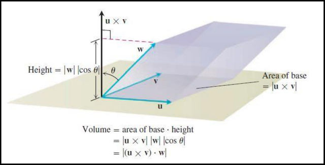
Figure 5.5: The number |(u × v) · w| is the volume of a parallelepiped

Figure 5.5: The number |(u × v) · w| is the volume of a parallelepiped.

By treating the planes of v\mathbf{v} and w\mathbf{w} and of w\mathbf{w} and u\mathbf{u} as the base planes of the parallelepiped determined by u\mathbf{u}, v\mathbf{v}, and w\mathbf{w}, we see that

(u×v)⋅w=(v×w)⋅u=(w×u)⋅v.(\mathbf{u} \times \mathbf{v})\cdot\mathbf{w} = (\mathbf{v} \times \mathbf{w})\cdot\mathbf{u} = (\mathbf{w} \times \mathbf{u})\cdot\mathbf{v}.

Since the dot product is commutative, we also have

(u×v)⋅w=u⋅(v×w).(\mathbf{u} \times \mathbf{v})\cdot\mathbf{w} = \mathbf{u}\cdot(\mathbf{v} \times \mathbf{w}).

The triple scalar product can be evaluated as a determinant:

(u×v)⋅w=[∣u2u3v2v3∣i−∣u1u3v1v3∣j+∣u1u2v1v2∣k]⋅w=w1∣u2u3v2v3∣−w2∣u1u3v1v3∣+w3∣u1u2v1v2∣=∣u1u2u3v1v2v3w1w2w3∣.\begin{aligned} (\mathbf{u} \times \mathbf{v})\cdot\mathbf{w} &= \left[\begin{vmatrix} u_2 & u_3 \\ v_2 & v_3 \end{vmatrix}\mathbf{i} - \begin{vmatrix} u_1 & u_3 \\ v_1 & v_3 \end{vmatrix}\mathbf{j} + \begin{vmatrix} u_1 & u_2 \\ v_1 & v_2 \end{vmatrix}\mathbf{k}\right]\cdot\mathbf{w} \\ &= w_1\begin{vmatrix} u_2 & u_3 \\ v_2 & v_3 \end{vmatrix} - w_2\begin{vmatrix} u_1 & u_3 \\ v_1 & v_3 \end{vmatrix} + w_3\begin{vmatrix} u_1 & u_2 \\ v_1 & v_2 \end{vmatrix} \\ &= \begin{vmatrix} u_1 & u_2 & u_3 \\ v_1 & v_2 & v_3 \\ w_1 & w_2 & w_3 \end{vmatrix}. \end{aligned}

Example 5.7​

Find the volume of the box (parallelepiped) determined by u=i+2j−k\mathbf{u} = \mathbf{i} + 2\mathbf{j} - \mathbf{k}, v=−2i+3k\mathbf{v} = -2\mathbf{i} + 3\mathbf{k}, and w=7j−4k\mathbf{w} = 7\mathbf{j} - 4\mathbf{k}.

Solution

Using the rule for calculating determinants, we find

(u×v)⋅w=∣12−1−20307−4∣=−23.(\mathbf{u} \times \mathbf{v})\cdot\mathbf{w} = \begin{vmatrix} 1 & 2 & -1 \\ -2 & 0 & 3 \\ 0 & 7 & -4 \end{vmatrix} = -23.

The volume is ∣(u×v)⋅w∣=23\lvert(\mathbf{u} \times \mathbf{v})\cdot\mathbf{w}\rvert = 23 units cubed.

Exercises​

Find the volume of the parallelepiped (box) determined by u, v, and w.

u\mathbf{u}v\mathbf{v}w\mathbf{w}
1)2i2\mathbf{i}2j2\mathbf{j}2k2\mathbf{k}
2)i−j+k\mathbf{i} - \mathbf{j} + \mathbf{k}2i+j−2k2\mathbf{i} + \mathbf{j} - 2\mathbf{k}−i+2j−k-\mathbf{i} + 2\mathbf{j} - \mathbf{k}
3)2i+j2\mathbf{i} + \mathbf{j}2i−j+k2\mathbf{i} - \mathbf{j} + \mathbf{k}i+2k\mathbf{i} + 2\mathbf{k}

5.2.5 Interpretation of the Directional Derivatives & Gradient​

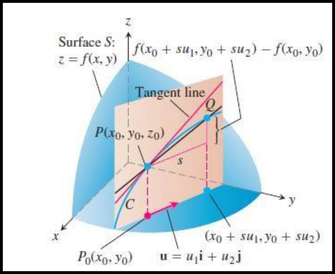
Figure 5.6: Interpretation of Directional Derivatives

Figure 5.6: Interpretation of Directional Derivatives.

From the Figure 5.6, the slope of curve C at Po is (Duf)Po in which it generalizes two partial derivatives. We can now ask for the rate of change of ff in any direction u\mathbf{u}, not just the directions i\mathbf{i} and j\mathbf{j}.

For a physical interpretation of the directional derivative, suppose that T=f(x,y)T = f(x, y) is the temperature at each point (x,y)(x, y) over a region in the plane. Then f(xo,yo)f(x_o, y_o) is the temperature at the point Po(xo,yo)P_o (x_o, y_o) and (Duf)Po(D_uf)_{P_o} is the instantaneous rate of change of the temperature at PoP_o stepping off in the direction u\mathbf{u}.

Properties of the Directional Derivative Duf=∇f⋅u=∣∇f∣cos⁡θD_{\mathbf{u}}f = \nabla f \cdot \mathbf{u} = \lvert\nabla f\rvert\cos\theta
  1. The function ff increases most rapidly when cos⁡θ=1\cos\theta = 1 or when θ=0\theta = 0 and u\mathbf{u} is the direction of ∇f\nabla f. That is, at each point PP in its domain, ff increases most rapidly in the direction of the gradient vector ∇f\nabla f at PP. The derivative in this direction is Duf=∣∇f∣cos⁡(0)=∣∇f∣.D_{\mathbf{u}}f = \lvert\nabla f\rvert\cos(0) = \lvert\nabla f\rvert.
  2. Similarly, ff decreases most rapidly in the direction of −∇f-\nabla f. The derivative in this direction is Duf=∣∇f∣cos⁡(π)=−∣∇f∣D_{\mathbf{u}}f = \lvert\nabla f\rvert\cos(\pi) = -\lvert\nabla f\rvert.
  3. Any direction u\mathbf{u} orthogonal to a gradient ∇f≠0\nabla f \neq 0 is a direction of zero change in ff because θ\theta then equals π/2\pi/2 and Duf=∣∇f∣cos⁡(π/2)=∣∇f∣⋅0=0.D_{\mathbf{u}}f = \lvert\nabla f\rvert\cos(\pi/2) = \lvert\nabla f\rvert\cdot 0 = 0.

Example 5.8​

(a) Find the derivative of f(x,y,z)=x3−xy2−zf(x,y,z) = x^3 - xy^2 - z at P0(1,1,0)P_0(1, 1, 0) in the direction of v=2i−3j+6k\mathbf{v} = 2\mathbf{i} - 3\mathbf{j} + 6\mathbf{k}.

(b) In what directions does ff change most rapidly at P0P_0, and what are the rates of change in these directions?

Solution

(a) The direction of v\mathbf{v} is obtained by dividing v\mathbf{v} by its length:

∣v∣=(2)2+(−3)2+(6)2=49=7\lvert\mathbf{v}\rvert = \sqrt{(2)^2 + (-3)^2 + (6)^2} = \sqrt{49} = 7

u=v∣v∣=27i−37j+67k.\mathbf{u} = \frac{\mathbf{v}}{\lvert\mathbf{v}\rvert} = \frac{2}{7}\mathbf{i} - \frac{3}{7}\mathbf{j} + \frac{6}{7}\mathbf{k}.

The partial derivatives of ff at P0P_0 are

fx=(3x2−y2)(1,1,0)=2,fy=−2xy∣(1,1,0)=−2,fz=−1∣(1,1,0)=−1.f_x = (3x^2 - y^2)_{(1,1,0)} = 2, \qquad f_y = -2xy\lvert_{(1,1,0)} = -2, \qquad f_z = -1\lvert_{(1,1,0)} = -1.

The gradient of ff at P0P_0 is

∇f∣(1,1,0)=2i−2j−k.\nabla f\lvert_{(1,1,0)} = 2\mathbf{i} - 2\mathbf{j} - \mathbf{k}.

The derivative of ff at P0P_0 in the direction of v\mathbf{v} is therefore

(Duf)(1,1,0)=∇f∣(1,1,0)⋅u=(2i−2j−k)⋅(27i−37j+67k)=47+67−67=47.\begin{aligned} (D_{\mathbf{u}}f)_{(1,1,0)} &= \nabla f\lvert_{(1,1,0)}\cdot\mathbf{u} = (2\mathbf{i} - 2\mathbf{j} - \mathbf{k})\cdot\left(\frac{2}{7}\mathbf{i} - \frac{3}{7}\mathbf{j} + \frac{6}{7}\mathbf{k}\right) \\ &= \frac{4}{7} + \frac{6}{7} - \frac{6}{7} = \frac{4}{7}. \end{aligned}

(b) The function increases most rapidly in the direction of ∇f=2i−2j−k\nabla f = 2\mathbf{i} - 2\mathbf{j} - \mathbf{k} and decreases most rapidly in the direction of −∇f-\nabla f. The rates of change in the directions are, respectively,

∣∇f∣=(2)2+(−2)2+(−1)2=9=3and−∣∇f∣=−3.\lvert\nabla f\rvert = \sqrt{(2)^2 + (-2)^2 + (-1)^2} = \sqrt{9} = 3 \qquad \text{and} \qquad -\lvert\nabla f\rvert = -3.

Example 5.9​

Suppose that the temperature TT at each point (x,y,z)(x, y, z) in a region of space is given by

T=100−x2−y2−z2,T = 100 - x^2 - y^2 - z^2,

and that F(x,y,z)\mathbf{F}(x, y, z) is defined to be the gradient of TT. Find the vector field F\mathbf{F}.

Solution

The gradient field F\mathbf{F} is the field F=∇T=−2xi−2yj−2zk\mathbf{F} = \nabla T = -2x\mathbf{i} - 2y\mathbf{j} - 2z\mathbf{k}. At each point in space, the vector field F\mathbf{F} gives the direction for which the increase in temperature is greatest.

Exercises​

Find the directions in which the functions increase and decrease most rapidly at PoP_o. Then find the derivatives of the functions in these directions.

(a) f(x,y,z)=ln⁡xy+ln⁡yz+ln⁡xzf(x, y, z) = \ln xy + \ln yz + \ln xz, Po(1,1,1)P_o(1, 1, 1)

(b) g(x,y,z)=xey+z2g(x, y, z) = xe^y + z^2, Po(1,ln⁡2,1/2)P_o(1, \ln 2, 1/2)

(c) f(x,y,z)=(x/y)−yzf(x, y, z) = (x/y) - yz, Po(4,1,1)P_o(4, 1, 1)

5.2.6 Gradients, Tangents and Normal to Level Curves​

The streams flow perpendicular to the contours. The streams are following paths of steepest descent so the waters reach the ocean as quickly as possible. Therefore, the fastest instantaneous rate of change in a stream's elevation above sea level has a particular direction. In this section, you will see why this direction, called the "downhill" direction, is perpendicular to the contours.
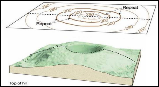
Figure 5.7: Contours of the hill

Figure 5.7: Contours of the hill

Based on above contours:

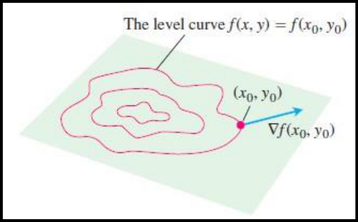
At every point (x0,y0)(x_0, y_0) in the domain of a differentiable function f(x,y)f(x, y), the gradient of ff is normal to the level curve through (x0,y0)(x_0, y_0) (Figure).

Figure 5.8: The gradient of a differentiable function of two variables at a point is always normal to the function's level curve through that point

Figure 5.8: The gradient of a differentiable function of two variables at a point is always normal to the function's level curve through that point.

Where it shows our observation that streams flow perpendicular to the contours in topographical maps (see Figure 5.7). Since the downflowing stream will reach its destination in the fastest way, it must flow in the direction of the negative gradient vectors from Property 2 for the directional derivative.

Now let us restrict our attention to the curves that pass through PoP_o (Figure Below). All the velocity vectors at PoP_o are orthogonal to ∇f\nabla f at PoP_o so the curves' tangent lines all lie in the plane through PoP_o normal to ∇f\nabla f. At every point along the curve, ∇f\nabla f is orthogonal to the curve's velocity vector.
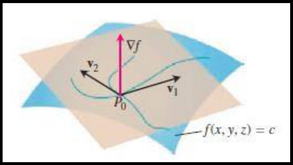
Figure Above: The gradient ∇f is orthogonal to the velocity vector of every smooth curve in the surface through P0

Figure Above: The gradient ∇f is orthogonal to the velocity vector of every smooth curve in the surface through P₀. The velocity vectors at P₀ therefore lie in a common plane, which we call the tangent plane at P₀.

We now define this plane.

Definitions

The tangent plane at the point P0(x0,y0,z0)P_0(x_0, y_0, z_0) on the level surface f(x,y,z)=cf(x, y, z) = c of a differentiable function ff is the plane through P0P_0 normal to ∇f∣P0\nabla f\lvert_{P_0}.

The normal line of the surface at P0P_0 is the line through P0P_0 parallel to ∇f∣P0\nabla f\lvert_{P_0}.

The tangent plane and normal line have the following equations:

Tangent Plane to f(x,y,z)=cf(x, y, z) = c at P0(x0,y0,z0)P_0(x_0, y_0, z_0)

fx(P0)(x−x0)+fy(P0)(y−y0)+fz(P0)(z−z0)=0(2)f_x(P_0)(x - x_0) + f_y(P_0)(y - y_0) + f_z(P_0)(z - z_0) = 0 \qquad (2)

Normal Line to f(x,y,z)=cf(x, y, z) = c at P0(x0,y0,z0)P_0(x_0, y_0, z_0)

x=x0+fx(P0)t,y=y0+fy(P0)t,z=z0+fz(P0)t(3)x = x_0 + f_x(P_0)t, \qquad y = y_0 + f_y(P_0)t, \qquad z = z_0 + f_z(P_0)t \qquad (3)

Example 5.10​

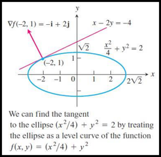
Find an equation for the tangent to the ellipse at the point (−2,1)(-2, 1).

x24+y2=2\frac{x^2}{4} + y^2 = 2

Solution

The ellipse is a level curve of the function

f(x,y)=x24+y2.f(x, y) = \frac{x^2}{4} + y^2.

The gradient of ff at (−2,1)(-2, 1) is

∇f∣(−2,1)=(x2i+2yj)(−2,1)=−i+2j.\nabla f\lvert_{(-2,1)} = \left(\frac{x}{2}\mathbf{i} + 2y\mathbf{j}\right)_{(-2,1)} = -\mathbf{i} + 2\mathbf{j}.

The tangent is the line

(−1)(x+2)+(2)(y−1)=0(-1)(x + 2) + (2)(y - 1) = 0

x−2y=−4.x - 2y = -4.

The ellipse x squared over 4 plus y squared equals 2 with its tangent line x - 2y = -4 at the point (-2, 1) and the gradient vector

We can find the tangent to the ellipse (x2/4)+y2=2(x^2/4) + y^2 = 2 by treating the ellipse as a level curve of the function f(x,y)=(x2/4)+y2f(x, y) = (x^2/4) + y^2

Example 5.11​

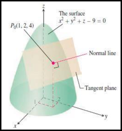
Find the tangent plane and normal line of the surface

f(x,y,z)=x2+y2+z−9=0A circular paraboloidf(x, y, z) = x^2 + y^2 + z - 9 = 0 \qquad \text{A circular paraboloid}

at the point P0(1,2,4)P_0(1, 2, 4).

Solution

The surface is shown in the figure below

The tangent plane is the plane through P0P_0 perpendicular to the gradient of ff at P0P_0. The gradient is

∇f∣P0=(2xi+2yj+k)(1,2,4)=2i+4j+k.\nabla f\lvert_{P_0} = (2x\mathbf{i} + 2y\mathbf{j} + \mathbf{k})_{(1,2,4)} = 2\mathbf{i} + 4\mathbf{j} + \mathbf{k}.

The tangent plane is therefore the plane

2(x−1)+4(y−2)+(z−4)=0,or2x+4y+z=14.2(x - 1) + 4(y - 2) + (z - 4) = 0, \qquad \text{or} \qquad 2x + 4y + z = 14.

The line normal to the surface at P0P_0 is

x=1+2t,y=2+4t,z=4+t.x = 1 + 2t, \qquad y = 2 + 4t, \qquad z = 4 + t.

The circular paraboloid x squared plus y squared plus z minus 9 equals 0 with its tangent plane and normal line at P0(1, 2, 4)

Exercises​

Find equations for the

(a) Tangent plane and (b) normal line at the point PoP_o on the given surface.

5.2.7 Application of Divergence and Curl​

Divergence at a given point measures the net flow out of a small box around the point, that is, it measures what is produced (source) or consumed (sink) at a given point in space.

For example, it is used to describe the flow of gas within a domain space. A gas is compressible, unlike a liquid, and the divergence of its velocity field measures to what extent it is expanding or compressing at each point. Intuitively, if a gas is expanding at the point (xo,yo)(x_o, y_o) the lines of flow would diverge there (hence the name) and, since the gas would be flowing out of a small rectangle about (xo,yo)(x_o, y_o), the divergence of F\mathbf{F} at (xo,yo)(x_o, y_o) would be positive. If the gas were compressing instead of expanding, the divergence would be negative.
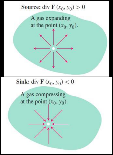
Figure 5.9: If a gas is expanding at a point the lines of flow have positive divergence; if the gas is compressing, the divergence is negative

Figure 5.9: If a gas is expanding at a point the lines of flow have positive divergence; if the gas is compressing, the divergence is negative. Otherwise, it will get zero.

Example 5.12​

Determine the divergence's characteristic of the vector fields; F(x,y)=3x2i−6xyjF(x, y) = 3x^2\mathbf{i} - 6xy\mathbf{j}

Solution
∇⋅F(x,y)=∂F1∂x+∂F2∂y=∂∂x3x2+∂∂y(−6xy)=6x−6x=0.\begin{aligned} \nabla \cdot F(x, y) &= \frac{\partial F_1}{\partial x} + \frac{\partial F_2}{\partial y} \\ &= \frac{\partial}{\partial x}3x^2 + \frac{\partial}{\partial y}(-6xy) = 6x - 6x = 0. \end{aligned}

A vector field with vanishing divergence is called a solenoidal vector field.

*In fluid dynamics, when the velocity field of a flowing liquid always has divergence equal to zero, as in those cases, the liquid is said to be incompressible.

If we think of the vector field as a velocity vector field of a fluid in a motion, the curl measures the rotation.

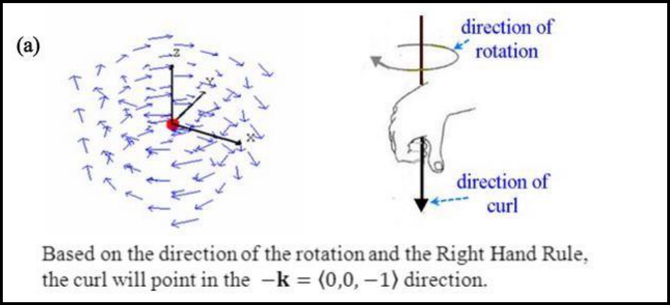
At a given point, the curl is a vector parallel to the axis of rotation of flow lines near the point, with direction determined by the Right Hand Rule.

Example 5.13​

Determine whether the curl of each vector field at the origin is the zero vector or points in the certain directions as ±i\pm\mathbf{i}, ±j\pm\mathbf{j}, ±k\pm\mathbf{k}.

Solution

(a)

Example 5.13(a): a vector field rotating about the z axis, with the right-hand rule giving the curl direction

Based on the direction of the rotation and the Right Hand Rule, the curl will point in the −k=⟨0,0,−1⟩-\mathbf{k} = \langle 0, 0, -1\rangle direction.

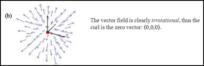
(b)

Example 5.13(b): a radially outward vector field, which is irrotational

The vector field is clearly irrotational, thus the curl is the zero vector: ⟨0,0,0⟩\langle 0, 0, 0\rangle.

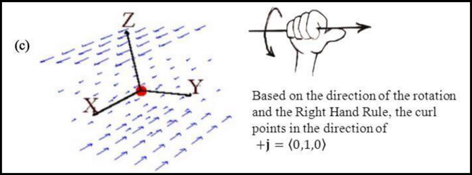
(c)

Example 5.13(c): a shearing vector field with the right-hand rule giving the curl direction

Based on the direction of the rotation and the Right Hand Rule, the curl points in the direction of +j=⟨0,1,0⟩+\mathbf{j} = \langle 0, 1, 0\rangle

Example 5.14​

The following vector fields represent the velocity of a gas flowing in the xyxy-plane. Find the divergence and curl of each vector field and interpret its physical meaning. Figure displays the vector fields.
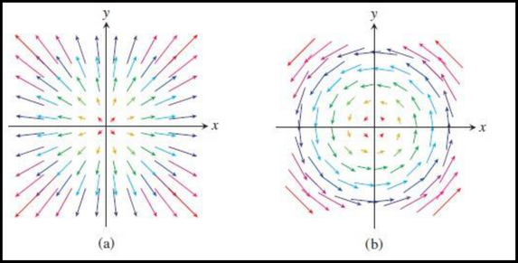
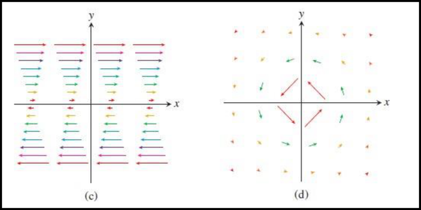
Example 5.14: velocity fields (a) uniform expansion and (b) rotation

Figure 5.10: Velocity fields of a gas flowing in the plane

Figure 5.10: Velocity fields of a gas flowing in the plane

Divergence​

Solution

(a) div F=∂∂x(cx)+∂∂y(cy)=2c\text{div } \mathbf{F} = \dfrac{\partial}{\partial x}(cx) + \dfrac{\partial}{\partial y}(cy) = 2c: If c>0c > 0, the gas is undergoing uniform expansion; if c<0c < 0, it is undergoing uniform compression.

(b) div F=∂∂x(−cy)+∂∂y(cx)=0\text{div } \mathbf{F} = \dfrac{\partial}{\partial x}(-cy) + \dfrac{\partial}{\partial y}(cx) = 0: The gas is neither expanding nor compressing.

(c) div F=∂∂x(y)=0\text{div } \mathbf{F} = \dfrac{\partial}{\partial x}(y) = 0: The gas is neither expanding nor compressing.

(d) div F=∂∂x(−yx2+y2)+∂∂y(xx2+y2)=2xy(x2+y2)2−2xy(x2+y2)2=0\text{div } \mathbf{F} = \dfrac{\partial}{\partial x}\left(\dfrac{-y}{x^2 + y^2}\right) + \dfrac{\partial}{\partial y}\left(\dfrac{x}{x^2 + y^2}\right) = \dfrac{2xy}{(x^2 + y^2)^2} - \dfrac{2xy}{(x^2 + y^2)^2} = 0: Again, the divergence is zero at all points in the domain of the velocity field.

Curl​

Solution

(a) Uniform expansion: (curl F)⋅k=∂∂x(cy)−∂∂y(cx)=0(\text{curl } \mathbf{F})\cdot\mathbf{k} = \dfrac{\partial}{\partial x}(cy) - \dfrac{\partial}{\partial y}(cx) = 0. The gas is not circulating at very small scales.

(b) Rotation: (curl F)⋅k=∂∂x(cx)−∂∂y(−cy)=2c(\text{curl } \mathbf{F})\cdot\mathbf{k} = \dfrac{\partial}{\partial x}(cx) - \dfrac{\partial}{\partial y}(-cy) = 2c. The constant circulation density indicates rotation at every point. If c>0c > 0, the rotation is counterclockwise; if c<0c < 0, the rotation is clockwise.

(c) Shear: (curl F)⋅k=−∂∂y(y)=−1(\text{curl } \mathbf{F})\cdot\mathbf{k} = -\dfrac{\partial}{\partial y}(y) = -1. The circulation density is constant and negative, so a paddle wheel floating in water undergoing such a shearing flow spins clockwise. The rate of rotation is the same at each point. The average effect of the fluid flow is to push fluid clockwise around each of the small circles shown in Figure 5.10.

(d) Whirlpool:

(curl F)⋅k=∂∂x(xx2+y2)−∂∂y(−yx2+y2)=y2−x2(x2+y2)2−y2−x2(x2+y2)2=0.(\text{curl } \mathbf{F})\cdot\mathbf{k} = \frac{\partial}{\partial x}\left(\frac{x}{x^2 + y^2}\right) - \frac{\partial}{\partial y}\left(\frac{-y}{x^2 + y^2}\right) = \frac{y^2 - x^2}{(x^2 + y^2)^2} - \frac{y^2 - x^2}{(x^2 + y^2)^2} = 0.

The circulation density is 0 at every point away from the origin (where the vector field is undefined and the whirlpool effect is taking place), and the gas is not circulating at any point for which the vector field is defined.