Lecture 6: Matrix Algebra for Non-Homogeneous Linear Algebraic System

Download the original PDF →

---

6.1 Introduction

A matrix is an array of $mn$ elements (where $m$ and $n$ are integers) arranged in $m$ rows and $n$ columns. The difference between matrix and column/ row vector is shown in Table 6.1.

Table 6.1 Matrix, column vector and row vector.

Matrix	Column vector (i.e. matrix with one column)	Row vector (i.e. matrix with one row)
$\mathbf{A} = \begin{bmatrix} a_{11} & a_{12} & a_{13} & \cdots & a_{1n} \\ a_{21} & a_{22} & a_{23} & \cdots & a_{2n} \\ a_{31} & a_{32} & a_{33} & \cdots & a_{3n} \\ \vdots & \vdots & \vdots & \ddots & \vdots \\ a_{m1} & a_{m2} & a_{m3} & \cdots & a_{mn} \end{bmatrix}$	$\mathbf{C} = \begin{Bmatrix} c_{11} \\ c_{21} \\ c_{31} \\ \vdots \\ c_{m1} \end{Bmatrix}$	$\mathbf{R} = \begin{Bmatrix} r_{11} & r_{12} & r_{13} & \cdots & r_{1n} \end{Bmatrix}$
Size $(\mathbf{A}) = m \times n$	Size $(\mathbf{C}) = m \times 1$	Size $(\mathbf{R}) = 1 \times n$

where $a_{mn}$ is the element of the matrix at $m^{th}$ row and $n^{th}$ column. If $m = n$, it is known as square matrix. Non-square matrix has $m \neq n$.

The common notation of matrix and vector is shown in Table 6.2:

Table 6.2 Common notation of matrix and vector.

Matrix	Vector
upper-case non-italic bold letter (e.g. $\mathbf{A} = \begin{bmatrix} 1 & 2 \\ 3 & 4 \end{bmatrix}$)	upper-case italic bold letter (e.g. $\boldsymbol{A} = \begin{Bmatrix} 1 \\ 3 \end{Bmatrix}$)
symbol in box bracket (e.g. $[A] = \begin{bmatrix} 1 & 2 \\ 3 & 4 \end{bmatrix}$)	symbol in curly bracket (e.g. $\{A\} = \begin{Bmatrix} 1 \\ 3 \end{Bmatrix}$)

Table 6.3 Type of matrices.

Zero/ Null Matrix	Symmetric Matrix	Diagonal Matrix
$\begin{bmatrix} 0 & 0 & 0 \\ 0 & 0 & 0 \\ 0 & 0 & 0 \end{bmatrix}$	$\begin{bmatrix} 5 & 1 & 2 \\ 1 & 3 & 7 \\ 2 & 7 & 8 \end{bmatrix}$ where $a_{ij} = a_{ji}$	$\begin{bmatrix} 5 & 0 & 0 \\ 0 & 3 & 0 \\ 0 & 0 & 8 \end{bmatrix}$ • All elements off the main diagonal are equal to 0.
Identity/ Unit Matrix	Upper Triangular matrix	Lower Triangular matrix
$\begin{bmatrix} 1 & 0 & 0 \\ 0 & 1 & 0 \\ 0 & 0 & 1 \end{bmatrix}$ • Diagonal matrix with element = 1	$\begin{bmatrix} 2 & -5 & 6 \\ 0 & 3 & 8 \\ 0 & 0 & 1 \end{bmatrix}$ • All the elements below main diagonal = 0	$\begin{bmatrix} 2 & 0 & 0 \\ 9 & 3 & 0 \\ 20 & -3 & 1 \end{bmatrix}$ • All the elements above main diagonal = 0
Banded Matrix	Tridiagonal Matrix	Anti-Symmetric / Skew-Symmetric Matrix
$\begin{bmatrix} a_{11} & a_{12} & a_{13} & 0 & 0 \\ a_{21} & a_{22} & a_{23} & a_{24} & 0 \\ a_{31} & a_{32} & a_{33} & a_{34} & a_{35} \\ 0 & a_{42} & a_{43} & a_{44} & a_{45} \\ 0 & 0 & a_{53} & a_{54} & a_{55} \end{bmatrix}$ • All elements = 0, except for a band centered on the main diagonal	$\begin{bmatrix} 1 & 3 & 0 & 0 \\ 5 & 2 & 9 & 0 \\ 0 & 6 & 5 & 1 \\ 0 & 0 & -3 & -9 \end{bmatrix}$ • Banded matrix that has bandwidth of 3.	$\begin{bmatrix} 5 & 1 & -2 \\ -1 & -3 & 7 \\ 2 & -7 & 8 \end{bmatrix}$ where $a_{ij} = -a_{ji}$

The basic operations of matrices such as trace, transpose, equality, addition/subtraction, scalar multiplication, transpose, multiplication, determinants, cofactor, adjoint, and inverse are provided in Table 6.4.

Table 6.4 Basic Operations of Matrices

Basic Matrix Algebra	Example
Trace	$\mathbf{F} = \begin{bmatrix} 4 & 13 & 3 \\ -2 & 19 & 1 \\ 3 & 2 & 0 \end{bmatrix}$ Trace (F) = Summation of diagonal element = $4+19+0=23$
Equality	$\mathbf{A} = \begin{bmatrix} 4 & 13 \\ -2 & 19 \end{bmatrix}$ ; $\mathbf{B} = \begin{bmatrix} 4 & 13 \\ -2 & 19 \end{bmatrix}$ ; $\mathbf{C} = \begin{bmatrix} 4 & 13 & 2 \\ -2 & 19 & 1 \end{bmatrix}$ $\therefore \mathbf{A} = \mathbf{B}$ ; $\mathbf{A} \neq \mathbf{C}$
Addition/Subtraction	$\mathbf{D} = \mathbf{A} + \mathbf{B} = \begin{bmatrix} 8 & 26 \\ -4 & 38 \end{bmatrix}$ $\mathbf{E} = \mathbf{A} - \mathbf{B} = \begin{bmatrix} 0 & 0 \\ 0 & 0 \end{bmatrix}$
Scalar Multiplication	$2\mathbf{D} = \begin{bmatrix} 16 & 52 \\ -8 & 76 \end{bmatrix}$
Transpose, $[\bullet]^T$	$\mathbf{C} = \begin{bmatrix} 4 & 13 & 2 \\ -2 & 19 & 1 \end{bmatrix}$ ; $\mathbf{C}^T = \begin{bmatrix} 4 & -2 \\ 13 & 19 \\ 2 & 1 \end{bmatrix}$
Matrix Multiplication Note: $\mathbf{AB} \neq \mathbf{BA}$	$\begin{bmatrix} 3 & 1 \\ 8 & 6 \\ 0 & 4 \end{bmatrix}_{(\text{Size 3x2})} \begin{bmatrix} 5 & 9 \\ 7 & 2 \end{bmatrix}_{(\text{Size 2x2})} = \begin{bmatrix} 22 & 29 \\ 82 & 84 \\ 28 & 8 \end{bmatrix}_{(\text{Size 3x2})}$ $\begin{bmatrix} 5 & 9 \\ 7 & 2 \end{bmatrix}_{(\text{Size 2x2})} \begin{bmatrix} 3 & 1 \\ 8 & 6 \\ 0 & 4 \end{bmatrix}_{(\text{Size 3x2})} = \text{error}$ (because non-equal interior dimensions)
Determinant, $\lvert\bullet\rvert$ Note: $\lvert\bullet\rvert$ is determinant, not absolute in this case. Note: It is inefficient to calculate determinant manually for 4x4 matrix and above.	$\mathbf{A} = \begin{bmatrix} 4 & 13 \\ -2 & 19 \end{bmatrix}$ ; $\lvert\mathbf{A}\rvert = \begin{vmatrix} 4 & 13 \\ -2 & 19 \end{vmatrix} = 4(19) - (-2)(13) = 102$ $\mathbf{F} = \begin{bmatrix} 4 & 13 & 3 \\ -2 & 19 & 1 \\ 3 & 2 & 0 \end{bmatrix}$ ; $\mathbf{G} = \begin{bmatrix} 4 & 13 & 3 & 3 \\ -2 & 19 & 1 & 1 \\ 3 & 2 & 0 & 0 \\ 0 & 2 & 1 & 0 \end{bmatrix}$ $\lvert\mathbf{F}\rvert = \begin{vmatrix} 4 & 13 & 3 \\ -2 & 19 & 1 \\ 3 & 2 & 0 \end{vmatrix} = 4\begin{vmatrix} 19 & 1 \\ 2 & 0 \end{vmatrix} - 13\begin{vmatrix} -2 & 1 \\ 3 & 0 \end{vmatrix} + 3\begin{vmatrix} -2 & 19 \\ 3 & 2 \end{vmatrix} = -152$ $\lvert\mathbf{G}\rvert = \begin{vmatrix} 4 & 13 & 3 & 3 \\ -2 & 19 & 1 & 1 \\ 3 & 2 & 0 & 0 \\ 0 & 2 & 1 & 0 \end{vmatrix} = 4\begin{vmatrix} 19 & 1 & 1 \\ 2 & 0 & 0 \\ 2 & 1 & 0 \end{vmatrix} - 13\begin{vmatrix} -2 & 1 & 1 \\ 3 & 0 & 0 \\ 0 & 1 & 0 \end{vmatrix} + 3\begin{vmatrix} -2 & 19 & 1 \\ 3 & 2 & 0 \\ 0 & 2 & 0 \end{vmatrix} - 3\begin{vmatrix} -2 & 19 & 1 \\ 3 & 2 & 0 \\ 0 & 2 & 1 \end{vmatrix}$ $= 4(2) - 13(3) + 3(6) - 3(-55) = 152$
Cofactor & Adjoint Note: adjoint = cofactor$^T$ Note: It is inefficient to calculate cofactor & adjoint manually for 4x4 matrix and above.	$\mathbf{A} = \begin{bmatrix} 4 & 13 \\ -2 & 19 \end{bmatrix}$ ; cofactor$(\mathbf{A}) = \begin{bmatrix} \lvert 19 \rvert & -\lvert -2 \rvert \\ -\lvert 13 \rvert & \lvert 4 \rvert \end{bmatrix} = \begin{bmatrix} 19 & 2 \\ -13 & 4 \end{bmatrix}$ adjoint$(\mathbf{A}) = (\text{cofactor}(\mathbf{A}))^T = \begin{bmatrix} 19 & 2 \\ -13 & 4 \end{bmatrix}^T = \begin{bmatrix} 19 & -13 \\ 2 & 4 \end{bmatrix}$ $\mathbf{F} = \begin{bmatrix} 4 & 13 & 3 \\ -2 & 19 & 1 \\ 3 & 2 & 0 \end{bmatrix}$ ; cofactor$(\mathbf{F}) = \begin{bmatrix} \begin{vmatrix} 19 & 1 \\ 2 & 0 \end{vmatrix} & -\begin{vmatrix} -2 & 1 \\ 3 & 0 \end{vmatrix} & \begin{vmatrix} -2 & 19 \\ 3 & 2 \end{vmatrix} \\ -\begin{vmatrix} 13 & 3 \\ 2 & 0 \end{vmatrix} & \begin{vmatrix} 4 & 3 \\ 3 & 0 \end{vmatrix} & -\begin{vmatrix} 4 & 13 \\ 3 & 2 \end{vmatrix} \\ \begin{vmatrix} 13 & 3 \\ 19 & 1 \end{vmatrix} & -\begin{vmatrix} 4 & 3 \\ -2 & 1 \end{vmatrix} & \begin{vmatrix} 4 & 13 \\ -2 & 19 \end{vmatrix} \end{bmatrix} = \begin{bmatrix} -2 & 3 & -61 \\ 6 & -9 & 31 \\ -44 & -10 & 102 \end{bmatrix}$ adjoint$(\mathbf{F}) = \begin{bmatrix} -2 & 6 & -44 \\ 3 & -9 & -10 \\ -61 & 31 & 102 \end{bmatrix}$ $\mathbf{G} = \begin{bmatrix} 4 & 13 & 3 & 3 \\ -2 & 19 & 1 & 1 \\ 3 & 2 & 0 & 0 \\ 0 & 2 & 1 & 0 \end{bmatrix}$ ; cofactor$(\mathbf{G}) = \begin{bmatrix} \begin{vmatrix} 19 & 1 & 1 \\ 2 & 0 & 0 \\ 2 & 1 & 0 \end{vmatrix} & -\begin{vmatrix} -2 & 1 & 1 \\ 3 & 0 & 0 \\ 0 & 1 & 0 \end{vmatrix} & \begin{vmatrix} -2 & 19 & 1 \\ 3 & 2 & 0 \\ 0 & 2 & 0 \end{vmatrix} & -\begin{vmatrix} -2 & 19 & 1 \\ 3 & 2 & 0 \\ 0 & 2 & 1 \end{vmatrix} \\ -\begin{vmatrix} 13 & 3 & 3 \\ 2 & 0 & 0 \\ 2 & 1 & 0 \end{vmatrix} & \begin{vmatrix} 4 & 3 & 3 \\ 3 & 0 & 0 \\ 0 & 1 & 0 \end{vmatrix} & -\begin{vmatrix} 4 & 13 & 3 \\ 3 & 2 & 0 \\ 0 & 2 & 0 \end{vmatrix} & \begin{vmatrix} 4 & 13 & 3 \\ 3 & 2 & 0 \\ 0 & 2 & 1 \end{vmatrix} \\ \begin{vmatrix} 13 & 3 & 3 \\ 19 & 1 & 1 \\ 2 & 1 & 0 \end{vmatrix} & -\begin{vmatrix} 4 & 3 & 3 \\ -2 & 1 & 1 \\ 0 & 1 & 0 \end{vmatrix} & \begin{vmatrix} 4 & 13 & 3 \\ -2 & 19 & 1 \\ 0 & 2 & 0 \end{vmatrix} & -\begin{vmatrix} 4 & 13 & 3 \\ -2 & 19 & 1 \\ 0 & 2 & 1 \end{vmatrix} \\ -\begin{vmatrix} 13 & 3 & 3 \\ 19 & 1 & 1 \\ 2 & 0 & 0 \end{vmatrix} & \begin{vmatrix} 4 & 3 & 3 \\ -2 & 1 & 1 \\ 3 & 0 & 0 \end{vmatrix} & -\begin{vmatrix} 4 & 13 & 3 \\ -2 & 19 & 1 \\ 3 & 2 & 0 \end{vmatrix} & \begin{vmatrix} 4 & 13 & 3 \\ -2 & 19 & 1 \\ 3 & 2 & 0 \end{vmatrix} \end{bmatrix}$ cofactor$(\mathbf{G}) = \begin{bmatrix} 2 & -3 & 6 & 55 \\ -6 & 9 & -18 & -13 \\ 44 & 10 & -20 & -82 \\ 0 & 0 & 152 & -152 \end{bmatrix}$ ; adjoint$(\mathbf{G}) = \begin{bmatrix} 2 & -6 & 44 & 0 \\ -3 & 9 & 10 & 0 \\ 6 & -18 & -20 & 152 \\ 55 & -13 & -82 & -152 \end{bmatrix}$
Inverse, $[\bullet]^{-1}$	$\mathbf{A} = \begin{bmatrix} 4 & 13 \\ -2 & 19 \end{bmatrix}$ ; $\mathbf{A}^{-1} = \dfrac{1}{\lvert\mathbf{A}\rvert}\,adjoint(\mathbf{A}) = \dfrac{1}{102}\begin{bmatrix} 19 & -13 \\ 2 & 4 \end{bmatrix}$ $\mathbf{F} = \begin{bmatrix} 4 & 13 & 3 \\ -2 & 19 & 1 \\ 3 & 2 & 0 \end{bmatrix}$ ; $\mathbf{F}^{-1} = \dfrac{1}{\lvert\mathbf{F}\rvert}\,adjoint(\mathbf{F}) = \dfrac{1}{-152}\begin{bmatrix} -2 & 6 & -44 \\ 3 & -9 & -10 \\ -61 & 31 & 102 \end{bmatrix}$ $\mathbf{G} = \begin{bmatrix} 4 & 13 & 3 & 3 \\ -2 & 19 & 1 & 1 \\ 3 & 2 & 0 & 0 \\ 0 & 2 & 1 & 0 \end{bmatrix}$ ; $\mathbf{G}^{-1} = \dfrac{1}{\lvert\mathbf{G}\rvert}\,adjoint(\mathbf{G}) = \dfrac{1}{152}\begin{bmatrix} 2 & -6 & 44 & 0 \\ -3 & 9 & 10 & 0 \\ 6 & -18 & -20 & 152 \\ 55 & -13 & -82 & -152 \end{bmatrix}$
Augmentation	$0.1x_1 + 7x_2 - 0.3x_3 = -19.3$ $3x_1 - 0.1x_2 - 0.2x_3 = 7.85$ $0.3x_1 - 0.2x_2 + 10x_3 = 71.4$ (i) Conventional Matrix form $\begin{bmatrix} 0.1 & 7 & -0.3 \\ 3 & -0.1 & -0.2 \\ 0.3 & -0.2 & 10 \end{bmatrix}\begin{Bmatrix} x_1 \\ x_2 \\ x_3 \end{Bmatrix} = \begin{Bmatrix} -19.3 \\ 7.85 \\ 71.4 \end{Bmatrix}$ (ii) Augmented Matrix form $\left[\begin{array}{ccccc} 0.1 & 7 & -0.3 & \vert & -19.3 \\ 3 & -0.1 & -0.2 & \vert & 7.85 \\ 0.3 & -0.2 & 10 & \vert & 71.4 \end{array}\right]$

---

6.2 Solving Non-Homogeneous System of Linear Equations

Multicomponent systems result in $n$ set(s) of mathematical equations that must be solved simultaneously. It can be represented by the following matrix format: $[A]\{X\} = \{B\}$. If $\{B\} \neq \{0\}$, it is known as non-homogeneous system of linear equations. In this study, several methods used to solve the unknown $\{X\}$ by using the $[A]$ & non-zero $\{B\}$ will be discussed next.

Linear Algebraic Equations	Coefficient Matrix, $[A]$	Unknown, $\{X\}$	Non-zero $\{B\}$
$4x_1 + 13x_2 = 8$ $-2x_1 + 19x_2 = 2$ $n=2$ where 2 sets of eqns. are given to solve $x_1$ & $x_2$ respectively.	$\begin{bmatrix} 4 & 13 \\ -2 & 19 \end{bmatrix}$	$\begin{Bmatrix} x_1 \\ x_2 \end{Bmatrix}$	$\begin{Bmatrix} 8 \\ 2 \end{Bmatrix}$
$0.5x_1 + 2.5x_2 - 9x_3 = -6$ $-4.5x_1 + 3.5x_2 - 2x_3 = 5$ $-8x_1 - 9x_2 + 22x_3 = 2$ $n=3$ where 3 sets of eqns. are given to solve $x_1$ , $x_2$ and $x_3$ respectively.	$\begin{bmatrix} 0.5 & 2.5 & -9 \\ -4.5 & 3.5 & -2 \\ -8 & -9 & 22 \end{bmatrix}$	$\begin{Bmatrix} x_1 \\ x_2 \\ x_3 \end{Bmatrix}$	$\begin{Bmatrix} -6 \\ 5 \\ 2 \end{Bmatrix}$

For $n \leq 3$, methods frequently used to solve the non-homogeneous system of linear equations are given below:

• (i) Matrix Inversion (Moderate efficiency for $n = 3$ & high efficiency for $n = 2$)
• (ii) Graphical method (Less efficiency but useful for visualizing & enhancing intuition)
• (iii) Cramer's rule (High efficiency for $n \leq 3$ - Main Focus)
• (iv) Method of elimination (Less efficiency)

However, method (i)- (iv) are less efficiency for $n > 3$, thus more advanced methods are introduced:

• (a) Gaussian Elimination (Naïve vs Partial Pivoting) --- Main Focus
• (b) LU Decomposition --- Out of scope
• (c) Thomas algorithm --- Out of scope
• (d) Gauss Seidel Method --- Out of scope

6.2.1 Matrix Inversion Approach

$[A]\{X\} = \{B\}$

If $[A]$ is a square and non-singular matrix, $[A][A]^{-1} = [A]^{-1}[A] = [I]$

$\{X\} = [A]^{-1}\{B\}$

Solution

$\mathbf{A} = \begin{bmatrix} 4 & 13 \\ -2 & 19 \end{bmatrix}; \quad \mathbf{A}^{-1} = \frac{1}{\lvert\mathbf{A}\rvert}\,adjoint(\mathbf{A}) = \frac{1}{102}\begin{bmatrix} 19 & -13 \\ 2 & 4 \end{bmatrix}; \quad \{X\} = \frac{1}{102}\begin{bmatrix} 19 & -13 \\ 2 & 4 \end{bmatrix}\begin{Bmatrix} 8 \\ 2 \end{Bmatrix} = \begin{Bmatrix} 126/102 \\ 24/102 \end{Bmatrix}$

6.2.2 Graphical Method

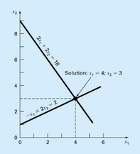
Rearrange the equations into linear plot format and then plot it.

Original linear equations	$a_{11}x_1 + a_{12}x_2 = b_1$ $a_{21}x_1 + a_{22}x_2 = b_2$	$3x_1 + 2x_2 = 18$ $-x_1 + 2x_2 = 2$
Linear plot format $x_2 = mx_1 + c$ where $m = slope$ ; $c = intercept$	$x_2 = -\left(\dfrac{a_{11}}{a_{12}}\right)x_1 + \left(\dfrac{b_1}{a_{12}}\right)$ $x_2 = -\left(\dfrac{a_{21}}{a_{22}}\right)x_1 + \left(\dfrac{b_2}{a_{22}}\right)$	$x_2 = -\left(\dfrac{3}{2}\right)x_1 + \left(\dfrac{18}{2}\right)$ $x_2 = -\left(\dfrac{-1}{2}\right)x_1 + \left(\dfrac{2}{2}\right)$

Using graphical method, the solution that satisfies both equations is the intersection point.

Solution

Graphical method: the two lines intersect at the solution point x1 = 4, x2 = 3.

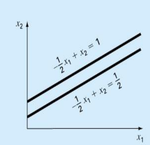
For singular system, the slopes of the equations are equal (or zero determinant), and it leads to

• (a) No solution case when there is no intersection between the lines or
• (b) Infinite solutions case when there are infinite intersection points between the lines.

(a) No solution case	(b) Infinite solutions case
$x_2 = +\left(\dfrac{1}{2}\right)x_1 + (1)$ $x_2 = +\left(\dfrac{1}{2}\right)x_1 + \left(\dfrac{1}{2}\right)$	$x_2 = +\left(\dfrac{1}{2}\right)x_1 + (1)$ $x_2 = +\left(\dfrac{1}{2}\right)x_1 + (1)$
Diff of slope $= \begin{vmatrix} -\dfrac{1}{2} & 1 \\ -\dfrac{1}{2} & 1 \end{vmatrix} = -\dfrac{1}{2} - \left(-\dfrac{1}{2}\right) = 0$	Diff of slope $= \begin{vmatrix} -\dfrac{1}{2} & 1 \\ -1 & 2 \end{vmatrix} = -1 - (-1) = 0$

(a) No solution case: the two lines never meet.

(b) Infinite solutions case: the two lines coincide.

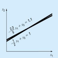
For ill-conditioned system (also known as ill-posed system), the slopes of the equations are almost equal (or close-to-zero determinant), and it leads to

• (c) Many solutions case and it is sensitive to round-off error.

(c) Many solutions case

$x_2 = +\left(\frac{2.3}{5}\right)x_1 + (1.1)$ $x_2 = +\left(\frac{1}{2}\right)x_1 + (1)$

(c) Many solutions case: the lines are almost parallel.

$\text{Diff of slope, } \begin{vmatrix} -\dfrac{2.3}{5} & 1 \\ -\dfrac{1}{2} & 1 \end{vmatrix} = -0.46 - (-0.5) = 0.04 \approx 0$

6.2.3 Cramer's Rule

$\begin{bmatrix} a_{11} & a_{12} & a_{13} \\ a_{21} & a_{22} & a_{23} \\ a_{31} & a_{32} & a_{33} \end{bmatrix}\begin{Bmatrix} x_1 \\ x_2 \\ x_3 \end{Bmatrix} = \begin{Bmatrix} b_1 \\ b_2 \\ b_3 \end{Bmatrix}$

$x_1 = \frac{\begin{vmatrix} b_1 & a_{12} & a_{13} \\ b_2 & a_{22} & a_{23} \\ b_3 & a_{32} & a_{33} \end{vmatrix}}{\lvert A \rvert}, \qquad x_2 = \frac{\begin{vmatrix} a_{11} & b_1 & a_{13} \\ a_{21} & b_2 & a_{23} \\ a_{31} & b_3 & a_{33} \end{vmatrix}}{\lvert A \rvert}, \qquad x_3 = \frac{\begin{vmatrix} a_{11} & a_{12} & b_1 \\ a_{21} & a_{22} & b_2 \\ a_{31} & a_{32} & b_3 \end{vmatrix}}{\lvert A \rvert}$

For example,

Solution

$\begin{bmatrix} 0.3 & 0.52 & 1 \\ 0.5 & 1 & 1.9 \\ 0.1 & 0.3 & 0.5 \end{bmatrix}\begin{Bmatrix} x_1 \\ x_2 \\ x_3 \end{Bmatrix} = \begin{Bmatrix} -0.01 \\ 0.67 \\ -0.44 \end{Bmatrix}$

$x_1 = \frac{\begin{vmatrix} -0.01 & 0.52 & 1 \\ 0.67 & 1 & 1.9 \\ -0.44 & 0.3 & 0.5 \end{vmatrix}}{\begin{vmatrix} 0.3 & 0.52 & 1 \\ 0.5 & 1 & 1.9 \\ 0.1 & 0.3 & 0.5 \end{vmatrix}} = -14.9, \qquad x_2 = \frac{\begin{vmatrix} 0.3 & -0.01 & 1 \\ 0.5 & 0.67 & 1.9 \\ 0.1 & -0.44 & 0.5 \end{vmatrix}}{\begin{vmatrix} 0.3 & 0.52 & 1 \\ 0.5 & 1 & 1.9 \\ 0.1 & 0.3 & 0.5 \end{vmatrix}} = -29.5, \qquad x_3 = \frac{\begin{vmatrix} 0.3 & 0.52 & -0.01 \\ 0.5 & 1 & 0.67 \\ 0.1 & 0.3 & -0.44 \end{vmatrix}}{\begin{vmatrix} 0.3 & 0.52 & 1 \\ 0.5 & 1 & 1.9 \\ 0.1 & 0.3 & 0.5 \end{vmatrix}} = 19.8$

Limitation: Impractical for eqns ($n > 3$).

6.2.4 Method of Elimination (Or Substitution Method)

$\begin{bmatrix} 0.3 & 0.52 & 1 \\ 0.5 & 1 & 1.9 \\ 0.1 & 0.3 & 0.5 \end{bmatrix}\begin{Bmatrix} x_1 \\ x_2 \\ x_3 \end{Bmatrix} = \begin{Bmatrix} -0.01 \\ 0.67 \\ -0.44 \end{Bmatrix}$

• Step 1: $x_1 = \cdots$ in $x_2$ & $x_3$ terms for $1^{st}$ eqn

• Step 2: Substitute $x_1 = \cdots$ to $2^{nd}$ & $3^{rd}$ eqns.

  Obtain $x_2 = \cdots$ in $x_3$ term

• Step 3: Substitute $x_2 = \cdots$ to $3^{rd}$ eqn.

  Obtain $x_3$ solution

• Step 4: Back Substitute to obtain $x_1$ & $x_2$ solutions

Limitation: Extremely tedious to solve manually. However, the elimination approach can be extended and made more systematically to improve the efficiency such as Gauss Elimination method.

6.2.5 Naïve Gauss Elimination

It is an extension of the method of elimination which has a systematic scheme with forward elimination & back substitution procedure.

Forward elimination #1

$\begin{bmatrix} a_{11} & a_{12} & a_{13} \\ a_{21} & a_{22} & a_{23} \\ a_{31} & a_{32} & a_{33} \end{bmatrix}\begin{Bmatrix} x_1 \\ x_2 \\ x_3 \end{Bmatrix} = \begin{Bmatrix} b_1 \\ b_2 \\ b_3 \end{Bmatrix} \xrightarrow{\text{Forward elimination \#1}} \begin{bmatrix} a_{11} & a_{12} & a_{13} \\ 0 & a'_{22} & a'_{23} \\ 0 & a'_{32} & a'_{33} \end{bmatrix}\begin{Bmatrix} x_1 \\ x_2 \\ x_3 \end{Bmatrix} = \begin{Bmatrix} b_1 \\ b'_2 \\ b'_3 \end{Bmatrix}$

R1 is the pivot equation, where $a_{11}$ is the pivot element to turn $a'_{21}$ & $a'_{31}$ into 0

$R2' = R2 - R1 \times f_{21} \quad \text{where factor, } f_{21} = \frac{a_{21}}{a_{11}} \quad ; \text{ For example, } a'_{21} = a_{21} - a_{11}f_{21} = 0$

$R3' = R3 - R1 \times f_{31} \quad \text{where factor, } f_{31} = \frac{a_{31}}{a_{11}} \quad ; \text{ For example, } a'_{31} = a_{31} - a_{11}f_{31} = 0$

Forward elimination #2

$\begin{bmatrix} a_{11} & a_{12} & a_{13} \\ 0 & a'_{22} & a'_{23} \\ 0 & a'_{32} & a'_{33} \end{bmatrix}\begin{Bmatrix} x_1 \\ x_2 \\ x_3 \end{Bmatrix} = \begin{Bmatrix} b_1 \\ b'_2 \\ b'_3 \end{Bmatrix} \xrightarrow{\text{Forward elimination \#2}} \begin{bmatrix} a_{11} & a_{12} & a_{13} \\ 0 & a'_{22} & a'_{23} \\ 0 & 0 & a''_{33} \end{bmatrix}\begin{Bmatrix} x_1 \\ x_2 \\ x_3 \end{Bmatrix} = \begin{Bmatrix} b_1 \\ b'_2 \\ b''_3 \end{Bmatrix}$

R2 is the pivot equation, where $a'_{22}$ is the pivot element to turn $a''_{32}$ to be 0

$R3'' = R3' - R2' \times f_{32} \quad \text{where factor, } f_{32} = \frac{a'_{32}}{a'_{22}} \quad ; \text{ For example, } a''_{32} = a'_{32} - a'_{22}f_{32} = 0$

Note: $\bullet'$ and $\bullet''$ indicate change of value after first and second elimination procedures, respectively.

Back Substitution

$\begin{bmatrix} a_{11} & a_{12} & a_{13} \\ 0 & a'_{22} & a'_{23} \\ 0 & 0 & a''_{33} \end{bmatrix}\begin{Bmatrix} x_1 \\ x_2 \\ x_3 \end{Bmatrix} = \begin{Bmatrix} b_1 \\ b'_2 \\ b''_3 \end{Bmatrix} \xrightarrow{\text{Back substitution \#1}} \text{Solution, } x_3 = \frac{b''_3}{a''_{33}}$

$\begin{bmatrix} a_{11} & a_{12} & a_{13} \\ 0 & a'_{22} & a'_{23} \\ 0 & 0 & a''_{33} \end{bmatrix}\begin{Bmatrix} x_1 \\ x_2 \\ x_3 \end{Bmatrix} = \begin{Bmatrix} b_1 \\ b'_2 \\ b''_3 \end{Bmatrix} \xrightarrow{\text{Back substitution \#2}} \text{Solution, } x_2 = \frac{b'_2 - a'_{23}x_3}{a'_{22}}$

$\begin{bmatrix} a_{11} & a_{12} & a_{13} \\ 0 & a'_{22} & a'_{23} \\ 0 & 0 & a''_{33} \end{bmatrix}\begin{Bmatrix} x_1 \\ x_2 \\ x_3 \end{Bmatrix} = \begin{Bmatrix} b_1 \\ b'_2 \\ b''_3 \end{Bmatrix} \xrightarrow{\text{Back substitution \#3}} \text{Solution, } x_1 = \frac{b_1 - a_{12}x_2 - a_{13}x_3}{a_{11}}$

For example:

Solution

$\begin{bmatrix} 3 & -0.1 & -0.2 \\ 0.1 & 7 & -0.3 \\ 0.3 & -0.2 & 10 \end{bmatrix}\begin{Bmatrix} x_1 \\ x_2 \\ x_3 \end{Bmatrix} = \begin{Bmatrix} 7.85 \\ -19.3 \\ 71.4 \end{Bmatrix}$

$\overline{\text{Forward elimination \#1}}$

$R2' = R2 - R1 \times \frac{0.1}{3} \qquad \begin{bmatrix} 3 & -0.1 & -0.2 \\ 0 & 7.00333 & -0.293333 \\ 0 & -0.190000 & 10.0200 \end{bmatrix}\begin{Bmatrix} x_1 \\ x_2 \\ x_3 \end{Bmatrix} = \begin{Bmatrix} 7.85 \\ -19.5617 \\ 70.6150 \end{Bmatrix}$

$R3' = R3 - R1 \times \frac{0.3}{3}$

$\overline{\text{Forward elimination \#2}}$

$R3'' = R3' - R2' \times \frac{-0.19}{7.00333} \qquad \begin{bmatrix} 3 & -0.1 & -0.2 \\ 0 & 7.00333 & -0.293333 \\ 0 & 0 & 10.0120 \end{bmatrix}\begin{Bmatrix} x_1 \\ x_2 \\ x_3 \end{Bmatrix} = \begin{Bmatrix} 7.85 \\ -19.5617 \\ 70.0843 \end{Bmatrix}$

$\overline{\text{Back substitution \#1}} \qquad x_3 = \dfrac{70.0843}{10.0120} = 7.0000$

$\overline{\text{Back substitution \#2}} \qquad x_2 = \dfrac{-19.5617 - (-0.293333)(7.0000)}{7.00333} = -2.50000$

$\overline{\text{Back substitution \#3}} \qquad x_1 = \dfrac{7.85 - (-0.1)(-2.5) - (-0.2)(7)}{3} = 3.00000$

Limitation: Suffer the division by zero issue or the solution is sensitive to round-off error

For example,

Solution

$\begin{bmatrix} 0 & 2 & 3 \\ 4 & 6 & 7 \\ 2 & 1 & 6 \end{bmatrix}\begin{Bmatrix} x_1 \\ x_2 \\ x_3 \end{Bmatrix} = \begin{Bmatrix} 8 \\ -3 \\ 5 \end{Bmatrix}$

$\overline{\text{Forward elimination \#1}}$

$R2' = R2 - R1 \times \frac{4}{0} \qquad \text{Error!}$

$R3' = R3 - R1 \times \frac{2}{0}$

For example,

Solution

$\begin{bmatrix} 2 & 100000 \\ 1 & 1 \end{bmatrix}\begin{Bmatrix} x_1 \\ x_2 \end{Bmatrix} = \begin{Bmatrix} 100000 \\ 2 \end{Bmatrix}$

$\overline{\text{Forward elimination \#2}}$

$R2' = R2 - R1 \times \frac{1}{2}$

$\begin{bmatrix} 2 & 100000 \\ 0 & -49999 \end{bmatrix}\begin{Bmatrix} x_1 \\ x_2 \end{Bmatrix} = \begin{Bmatrix} 100000 \\ -49998 \end{Bmatrix}$

$\overline{\text{Back substitution \#1}} \qquad x_2 = 1$

$\overline{\text{Back substitution \#2}} \qquad x_1 = \dfrac{100000 - 100000x_2}{2} = 0$

Verification of solution:

LHS:	RHS:
$\begin{bmatrix} 2 & 100000 \\ 1 & 1 \end{bmatrix}\begin{Bmatrix} 0 \\ 1 \end{Bmatrix} = \begin{Bmatrix} 100000 \\ 1 \end{Bmatrix}$	$\begin{Bmatrix} 100000 \\ 2 \end{Bmatrix}$
$\therefore LHS \neq RHS$ as percentage of error, $\begin{Bmatrix} \%\,\text{error}_{b_1} \\ \%\,\text{error}_{b_2} \end{Bmatrix} = \begin{Bmatrix} \dfrac{100000-100000}{100000} \times 100\% \\ \dfrac{2-1}{2} \times 100\% \end{Bmatrix} = \begin{Bmatrix} 0\% \\ 50\% \end{Bmatrix}$

Thus, $\begin{Bmatrix} x_1 \\ x_2 \end{Bmatrix} = \begin{Bmatrix} 0 \\ 1 \end{Bmatrix}$ is a poor solution as it is different from the actual solution. The solution is sensitive to the round-off error which leads to high error discrepancy.

6.2.6 Gauss Elimination with Partial Pivoting (GEwPP)

The limitation of Naïve Gauss Elimination can be improved by using GEwPP that consists of scaling analysis & pivoting strategy:

(a) Scaling analysis: Indicates the requirement of having pivoting to avoid divide by zero issue.

$\begin{bmatrix} 2 & 100000 \\ 1 & 1 \end{bmatrix}\begin{Bmatrix} x_1 \\ x_2 \end{Bmatrix} = \begin{Bmatrix} 100000 \\ 2 \end{Bmatrix} \xrightarrow{\text{Scaling the coefficient matrix to have max value of 1}} \begin{bmatrix} 0.00002 & 1 \\ 1 & 1 \end{bmatrix}\begin{Bmatrix} x_1 \\ x_2 \end{Bmatrix} = \begin{Bmatrix} 1 \\ 2 \end{Bmatrix}$

pivot element is smaller

Rule of thumbs: If the pivot element is smaller than other rows, then pivoting is needed.

(b) Pivoting strategy: Switch row/ column to avoid pivot element to be zero or close to zero

(i) Naïve Gauss Elimination - Gaussian Elimination (GE) without pivoting strategy

$\begin{bmatrix} 2 & 100000 \\ 1 & 1 \end{bmatrix}\begin{Bmatrix} x_1 \\ x_2 \end{Bmatrix} = \begin{Bmatrix} 100000 \\ 2 \end{Bmatrix}$

Note: Previously we remain the original formulation and get poor solution after solving it.

(ii) Gauss Elimination with Partial Pivoting (GEwPP) -Switch row so that largest element is the pivot element (Main Focus).

$\begin{bmatrix} 0.00002 & 1 \\ 1 & 1 \end{bmatrix}\begin{Bmatrix} x_1 \\ x_2 \end{Bmatrix} = \begin{Bmatrix} 1 \\ 2 \end{Bmatrix} \xrightarrow{\text{Partial pivoting}} \begin{bmatrix} 1 & 1 \\ 0.00002 & 1 \end{bmatrix}\begin{Bmatrix} x_1 \\ x_2 \end{Bmatrix} = \begin{Bmatrix} 2 \\ 1 \end{Bmatrix}$

pivot element is the largest

Example of GEwPP

Solution

$\begin{bmatrix} 2 & 100000 \\ 1 & 1 \end{bmatrix}\begin{Bmatrix} x_1 \\ x_2 \end{Bmatrix} = \begin{Bmatrix} 100000 \\ 2 \end{Bmatrix}$

$\overline{\text{Scaling}} \qquad \begin{bmatrix} 0.00002 & 1 \\ 1 & 1 \end{bmatrix}\begin{Bmatrix} x_1 \\ x_2 \end{Bmatrix} = \begin{Bmatrix} 1 \\ 2 \end{Bmatrix} \qquad$ Note: Scaling indicates partial pivoting is needed

$\overline{\text{Partial Pivoting}} \qquad \begin{bmatrix} 1 & 1 \\ 0.00002 & 1 \end{bmatrix}\begin{Bmatrix} x_1 \\ x_2 \end{Bmatrix} = \begin{Bmatrix} 2 \\ 1 \end{Bmatrix} \qquad$ Note: Pivot element is the largest after PP.

$\begin{bmatrix} 1 & 1 \\ 0 & 1 \end{bmatrix}\begin{Bmatrix} x_1 \\ x_2 \end{Bmatrix} = \begin{Bmatrix} 2 \\ 1 \end{Bmatrix} \qquad \text{Note: Round-off error happens when we use approximate value}$

$\overline{\text{Back substitution \#1}} \qquad x_2 = 1$

$\overline{\text{Back substitution \#2}} \qquad x_1 = 2 - x_2 = 1$

Verification of solution:

LHS:	RHS:
$\begin{bmatrix} 2 & 100000 \\ 1 & 1 \end{bmatrix}\begin{Bmatrix} 1 \\ 1 \end{Bmatrix} = \begin{Bmatrix} 100002 \\ 2 \end{Bmatrix}$	$\begin{Bmatrix} 100000 \\ 2 \end{Bmatrix}$
$\therefore LHS \approx RHS$ as percentage of error, $\begin{Bmatrix} \%\,\text{error}_{b_1} \\ \%\,\text{error}_{b_2} \end{Bmatrix} = \begin{Bmatrix} \dfrac{\lvert 100000-100002 \rvert}{100000} \times 100\% \\ \dfrac{\lvert 2-2 \rvert}{2} \times 100\% \end{Bmatrix} = \begin{Bmatrix} 0.002\% \\ 0\% \end{Bmatrix}$

Thus, $\begin{Bmatrix} x_1 \\ x_2 \end{Bmatrix} = \begin{Bmatrix} 1 \\ 1 \end{Bmatrix}$ is an accurate solution as it is close to the actual solution. The solution is less sensitive to the round-off error by using the GEwPP, as compares to naïve GE.

Determinant analysis can be done before GEwPP to know if you have well-conditioned system or singular system. Precaution: scaling is performed to standardize matrix before calculating determinant.

Well-conditioned system, $\lvert\bullet\rvert \neq 0$	Singular system, $\lvert\bullet\rvert = 0$
$-1x_1 + 1x_2 + 2x_3 = 2$ $3x_1 - 1x_2 + 1x_3 = 6$ $-1x_1 + 3x_2 + 4x_3 = 4$ Unique solution for $\begin{Bmatrix} x_1 \\ x_2 \\ x_3 \end{Bmatrix}$ exists as $\begin{vmatrix} -\dfrac{1}{2} & \dfrac{1}{2} & 1 \\ 1 & -\dfrac{1}{3} & \dfrac{1}{3} \\ -\dfrac{1}{4} & \dfrac{3}{4} & 1 \end{vmatrix} = 0.4 \neq 0$	$-1x_1 + 1x_2 + 2x_3 = 2$ $3x_1 - 1x_2 + 1x_3 = 6$ $-2x_1 + 2x_2 + 4x_3 = 4$ $\begin{vmatrix} -\dfrac{1}{2} & \dfrac{1}{2} & 1 \\ 1 & -\dfrac{1}{3} & \dfrac{1}{3} \\ -\dfrac{2}{4} & \dfrac{2}{4} & 1 \end{vmatrix} = 0$	$-1x_1 + 1x_2 + 2x_3 = 2$ $3x_1 - 1x_2 + 1x_3 = 6$ $-2x_1 + 2x_2 + 4x_3 = 8$ We get no solution or infinite solutions for $\begin{Bmatrix} x_1 \\ x_2 \\ x_3 \end{Bmatrix}$, we can know either it is no solution or infinite solutions by using GEwPP.

Rule of thumb: Assume that $-0.1 \leq \lvert\bullet\rvert \leq 0.1$ is considered as ill-conditioned system in this study.

Example: Solving a well-conditioned system using GEwPP

$\begin{bmatrix} -1 & 1 & 2 \\ 3 & -1 & 1 \\ -1 & 3 & 4 \end{bmatrix}\begin{Bmatrix} x_1 \\ x_2 \\ x_3 \end{Bmatrix} = \begin{Bmatrix} 2 \\ 6 \\ 4 \end{Bmatrix}$

Solution

$\overline{\text{Scaling}} \qquad \left[\begin{array}{cccc} -1/2 & 1/2 & 1 & 1 \\ 1 & -1/3 & 1/3 & 2 \\ -1/4 & 3/4 & 1 & 1 \end{array}\right] \qquad \overline{\text{Pivoting}} \qquad \left[\begin{array}{cccc} 1 & -1/3 & 1/3 & 2 \\ -1/2 & 1/2 & 1 & 1 \\ -1/4 & 3/4 & 1 & 1 \end{array}\right]$

$\overline{\text{Forward elimination \#1}}$

$R2' = R2 - R1 \times \frac{\left(-\dfrac{1}{2}\right)}{1} \qquad \left[\begin{array}{cccc} 1 & -1/3 & 1/3 & 2 \\ 0 & 1/3 & 7/6 & 2 \\ 0 & 2/3 & 13/12 & 1.5 \end{array}\right]$

$R3' = R3 - R1 \times \frac{\left(-\dfrac{1}{4}\right)}{1}$

$\overline{\text{Scaling}} \qquad \left[\begin{array}{cccc} 1 & -1/3 & 1/3 & 2 \\ 0 & 2/7 & 1 & 12/7 \\ 0 & 8/13 & 1 & 18/13 \end{array}\right] \qquad \overline{\text{Pivoting}} \qquad \left[\begin{array}{cccc} 1 & -1/3 & 1/3 & 2 \\ 0 & 8/13 & 1 & 18/13 \\ 0 & 2/7 & 1 & 12/7 \end{array}\right]$

$\overline{\text{Forward elimination \#2}}$

$R3'' = R3' - R2' \times \frac{\left(\dfrac{2}{7}\right)}{\left(\dfrac{8}{13}\right)} \qquad \left[\begin{array}{cccc} 1 & -1/3 & 1/3 & 2 \\ 0 & 8/13 & 1 & 18/13 \\ 0 & 0 & 15/28 & 15/14 \end{array}\right]$

$\overline{\text{Back substitution}}$

$x_3 = \frac{15/14}{15/28} = 2$

$x_2 = \frac{18/13 - (1)x_3}{8/13} = -1$

$x_1 = \frac{2 - (-1/3)x_2 - (1/3)x_3}{1} = 1$

$\therefore \begin{Bmatrix} x_1 \\ x_2 \\ x_3 \end{Bmatrix} = \begin{Bmatrix} 1 \\ -1 \\ 2 \end{Bmatrix}$ is an accurate solution as LHS=RHS (verification).

Example: Solving a singular system (infinite solutions case) using GEwPP

$\begin{bmatrix} -1 & 1 & 2 \\ 3 & -1 & 1 \\ -2 & 2 & 4 \end{bmatrix}\begin{Bmatrix} x_1 \\ x_2 \\ x_3 \end{Bmatrix} = \begin{Bmatrix} 2 \\ 6 \\ 4 \end{Bmatrix}$

Solution

$\overline{\text{Scaling}} \qquad \left[\begin{array}{cccc} -1/2 & 1/2 & 1 & 1 \\ 1 & -1/3 & 1/3 & 2 \\ -2/4 & 2/4 & 1 & 1 \end{array}\right]$

$\overline{\text{Pivoting}} \qquad \left[\begin{array}{cccc} 1 & -1/3 & 1/3 & 2 \\ -1/2 & 1/2 & 1 & 1 \\ -2/4 & 2/4 & 1 & 1 \end{array}\right]$

$\overline{\text{Forward elimination \#1}}$

$R2' = R2 - R1 \times \frac{\left(-\dfrac{1}{2}\right)}{1} \qquad \left[\begin{array}{cccc} 1 & -1/3 & 1/3 & 2 \\ 0 & 1/3 & 7/6 & 2 \\ 0 & 1/3 & 7/6 & 2 \end{array}\right]$

$R3' = R3 - R1 \times \frac{\left(-\dfrac{2}{4}\right)}{1}$

$\overline{\text{Forward elimination \#2}}$

$R3'' = R3' - R2' \times \frac{\left(\dfrac{1}{3}\right)}{\left(\dfrac{1}{3}\right)} \qquad \left[\begin{array}{cccc} 1 & -1/3 & 1/3 & 2 \\ 0 & 1/3 & 7/6 & 2 \\ 0 & 0 & 0 & 0 \end{array}\right]$

$\overline{\text{Back substitution}} \qquad 0x_3 = 0$

$x_3 = t, \ where -\infty \leq t \leq \infty$

$x_2 = \frac{2 - (7/6)x_3}{1/3}$

$x_1 = \frac{2 - (-1/3)x_2 - (1/3)x_3}{1}$

$\therefore \begin{Bmatrix} x_1 \\ x_2 \\ x_3 \end{Bmatrix} = \begin{Bmatrix} \dfrac{2 - (-1/3)\left[\dfrac{2-(7/6)t}{1/3}\right] - (1/3)t}{1} \\ \dfrac{2-(7/6)t}{1/3} \\ t \end{Bmatrix}$

Infinite solutions that can satisfy the eqns.

Example: Solving a singular system (no solution case) using GEwPP

$\begin{bmatrix} -1 & 1 & 2 \\ 3 & -1 & 1 \\ -2 & 2 & 4 \end{bmatrix}\begin{Bmatrix} x_1 \\ x_2 \\ x_3 \end{Bmatrix} = \begin{Bmatrix} 2 \\ 6 \\ 8 \end{Bmatrix}$

Solution

$\overline{\text{Scaling}} \qquad \left[\begin{array}{cccc} -1/2 & 1/2 & 1 & 1 \\ 1 & -1/3 & 1/3 & 2 \\ -2/4 & 2/4 & 1 & 2 \end{array}\right]$

$\overline{\text{Pivoting}} \qquad \left[\begin{array}{cccc} 1 & -1/3 & 1/3 & 2 \\ -1/2 & 1/2 & 1 & 1 \\ -2/4 & 2/4 & 1 & 2 \end{array}\right]$

$\overline{\text{Forward elimination \#1}}$

$R2' = R2 - R1 \times \frac{\left(-\dfrac{1}{2}\right)}{1} \qquad \left[\begin{array}{cccc} 1 & -1/3 & 1/3 & 2 \\ 0 & 1/3 & 7/6 & 2 \\ 0 & 1/3 & 7/6 & 3 \end{array}\right]$

$R3' = R3 - R1 \times \frac{\left(-\dfrac{2}{4}\right)}{1}$

$\overline{\text{Forward elimination \#2}}$

$R3'' = R3' - R2' \times \frac{\left(\dfrac{1}{3}\right)}{\left(\dfrac{1}{3}\right)} \qquad \left[\begin{array}{cccc} 1 & -1/3 & 1/3 & 2 \\ 0 & 1/3 & 7/6 & 2 \\ 0 & 0 & 0 & 1 \end{array}\right]$

$\overline{\text{Back substitution}} \qquad 0x_3 = 1 \qquad \therefore \text{No solutions that satisfy the eqns.}$

---

6.3 Row Echelon Form, Reduced Row Echelon Form, Rank, & Linear Dependency

After the GEwPP, the coefficient matrix will be in the Row Echelon Form (REF). From the previous example, we obtain:

Well-conditioned system, $\lvert\bullet\rvert \neq 0$	Singular system, $\lvert\bullet\rvert = 0$
$-1x_1 + 1x_2 + 2x_3 = 2$ $3x_1 - 1x_2 + 1x_3 = 6$ $-1x_1 + 3x_2 + 4x_3 = 4$ Coefficient matrix, $[A] = \begin{bmatrix} -1 & 1 & 2 \\ 3 & -1 & 1 \\ -1 & 3 & 4 \end{bmatrix}$ Coefficient matrix after GEwPP is in REF, $[A]_{GEwPP} = \begin{bmatrix} 1 & -1/3 & 1/3 \\ 0 & 8/13 & 1 \\ 0 & 0 & 15/28 \end{bmatrix}$	$-1x_1 + 1x_2 + 2x_3 = 2$ $3x_1 - 1x_2 + 1x_3 = 6$ $-2x_1 + 2x_2 + 4x_3 = 4$ $-1x_1 + 1x_2 + 2x_3 = 2$ $3x_1 - 1x_2 + 1x_3 = 6$ $-2x_1 + 2x_2 + 4x_3 = 8$ Coefficient matrix, $[A] = \begin{bmatrix} -1 & 1 & 2 \\ 3 & -1 & 1 \\ -2 & 2 & 4 \end{bmatrix}$ Coefficient matrix after GEwPP is in REF, $[A]_{GEwPP} = \begin{bmatrix} 1 & -1/3 & 1/3 \\ 0 & 1/3 & 7/6 \\ 0 & 0 & 0 \end{bmatrix}$

REF has the following characteristics:

• Zero row(s) are always below non-zero rows if there is any.
• Pivot element of the non-zero rows at the bottom must be at the right of the pivot element above it.
• Non-unique; can be in different scale

REF can be further reduced to Reduced Row Echelon Form (RREF) by using Gauss-Jordan Elimination with Partial Pivoting (GJEwPP) as shown in the example below:

Solution

Well-conditioned system, $\lvert\bullet\rvert \neq 0$

Singular system, $\lvert\bullet\rvert = 0$

$[A]_{GEwPP} = \begin{bmatrix} 1 & -1/3 & 1/3 \\ 0 & 8/13 & 1 \\ 0 & 0 & 15/28 \end{bmatrix}$ $\overline{\text{Scale the pivot element to 1}}$ $R2 \to R2 \times \dfrac{13}{8}$ $R3 \to R3 \times \dfrac{28}{15}$ $\begin{bmatrix} 1 & -1/3 & 1/3 \\ 0 & 1 & 13/8 \\ 0 & 0 & 1 \end{bmatrix}$ $\overline{\text{Forward elimination}}$ $R1 \to R1 - R2 \times \dfrac{\left(-\dfrac{1}{3}\right)}{1}$ $\begin{bmatrix} 1 & 0 & 7/8 \\ 0 & 1 & 13/8 \\ 0 & 0 & 1 \end{bmatrix}$ $\overline{\text{Forward elimination}}$ $R1 \to R1 - R3 \times \dfrac{\left(\dfrac{7}{8}\right)}{1}$ $R2 \to R2 - R3 \times \dfrac{\left(\dfrac{13}{8}\right)}{1}$ $\begin{bmatrix} 1 & 0 & 0 \\ 0 & 1 & 0 \\ 0 & 0 & 1 \end{bmatrix}$

$[A]_{GEwPP} = \begin{bmatrix} 1 & -1/3 & 1/3 \\ 0 & 1/3 & 7/6 \\ 0 & 0 & 0 \end{bmatrix}$ $\overline{\text{Scale the pivot element to 1}}$ $R2 \to R2 \times 3$ $R3 \to R3 \times \dfrac{-1}{1.25}$ $\begin{bmatrix} 1 & -1/3 & 1/3 \\ 0 & 1 & 3.5 \\ 0 & 0 & 0 \end{bmatrix}$ $\overline{\text{Forward elimination}}$ $R1 \to R1 - R2 \times \dfrac{\left(-\dfrac{1}{3}\right)}{1}$ $\begin{bmatrix} 1 & 0 & 1.5 \\ 0 & 1 & 3.5 \\ 0 & 0 & 0 \end{bmatrix}$

RREF has the following characteristics:

• Also a REF
• Unique; Scale the pivot element to 1
• Element above the pivot element is 0

Once RREF is obtained, rank of a matrix can be evaluated by counting the number of non-zero rows of RREF. Note: Rank is the maximum number of linearly independent vector.

Well-conditioned system, $\lvert\bullet\rvert \neq 0$

Singular system, $\lvert\bullet\rvert = 0$

REF= $\begin{bmatrix} 1 & -1/3 & 1/3 \\ 0 & 8/13 & 1 \\ 0 & 0 & 15/28 \end{bmatrix}$ RREF= $\begin{bmatrix} 1 & 0 & 0 \\ 0 & 1 & 0 \\ 0 & 0 & 1 \end{bmatrix}$ Rank=3 It means that all the 3 equations given are linear independent, therefore finding 3 unknowns from 3 linear independent equations are possible. $-1x_1 + 1x_2 + 2x_3 = 2$ $3x_1 - 1x_2 + 1x_3 = 6$ $-1x_1 + 3x_2 + 4x_3 = 4$ $\therefore [A] = \text{Full rank matrix}$

REF= $\begin{bmatrix} 1 & -1/3 & 1/3 \\ 0 & 1/3 & 7/6 \\ 0 & 0 & 0 \end{bmatrix}$ RREF= $\begin{bmatrix} 1 & 0 & 1.5 \\ 0 & 1 & 3.5 \\ 0 & 0 & 0 \end{bmatrix}$ Rank=2 It means that only 2 out of 3 equations given are linear independent, therefore finding 3 unknowns from 2 linear independent equations are difficult. $-1x_1 + 1x_2 + 2x_3 = 2$ $3x_1 - 1x_2 + 1x_3 = 6$ $-2x_1 + 2x_2 + 4x_3 = 4$ $\therefore [A] = \text{Rank-deficient matrix}$

As a rule of thumbs, $n$ linearly independent equations are required to solve $n$ unknowns. To solve 3 unknowns, if we have less than 3 linearly independent equations, i.e. more unknowns than knowns, then we get the singular system issue.

---

6.4 Engineering Application of Non-Homogeneous System of Linear Equations

(a) Transform information into multiple linear algebraic equations to be solved simultaneously.

The amounts of metal, plastic, and rubber needed for electrical components types #1, #2, and #3 are shown in the following Table.

Component	Metal (g/ component)	Plastic (g/ component)	Rubber (g/ component)
1	15	0.25	1.0
2	17	0.33	1.2
3	19	0.42	1.6

Note: It is important for student to convert the information into multiple linear algebraic equations & matrix format.

If totals of 2120, 43.4 and 164 g of metal, plastic, and rubber respectively are available each day. How many components can be produced per day?

Solution

$15Comp_1 + 17Comp_2 + 19Comp_3 = 2120$ $0.25Comp_1 + 0.33Comp_2 + 0.42Comp_3 = 43.4$ $1.0Comp_1 + 1.2Comp_2 + 1.6Comp_3 = 164$

$\begin{bmatrix} 15 & 17 & 19 \\ 0.25 & 0.33 & 0.42 \\ 1.0 & 1.2 & 1.6 \end{bmatrix}\begin{Bmatrix} Comp_1 \\ Comp_2 \\ Comp_3 \end{Bmatrix} = \begin{Bmatrix} 2120 \\ 43.4 \\ 164 \end{Bmatrix}$

Then, it can be solved by using the GEwPP, Cramer's rule, etc.

(b) Electrical system

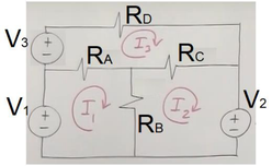
Electrical circuit with three loops.

Source: https://www.youtube.com/watch?v=2naaCxfbq_M

$\begin{bmatrix} R_A + R_B & -R_B & -R_A \\ -R_B & R_B + R_C & -R_C \\ -R_A & -R_C & R_A + R_C + R_D \end{bmatrix}\begin{Bmatrix} I_1 \\ I_2 \\ I_3 \end{Bmatrix} = \begin{Bmatrix} +V_1 \\ -V_2 \\ +V_3 \end{Bmatrix}$

Eg. If the resistance, $R$ and voltage, $V$ are given, estimate the output currents, $I$ of the 3 dof electrical circuit system.

Solution

$\begin{bmatrix} 4 + 2 & -2 & -4 \\ -2 & 2 + 8 & -8 \\ -4 & -8 & 4 + 6 + 8 \end{bmatrix}\begin{Bmatrix} I_1 \\ I_2 \\ I_3 \end{Bmatrix} = \begin{Bmatrix} 16 \\ -40 \\ 0 \end{Bmatrix}$

Note: The derivation of the eqns involves theory of circuit, thus it is not examined in this study.

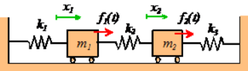
(c) Mechanical vibration system

Two degree-of-freedom mass-spring vibration system.

Source: https://www.brown.edu/Departments/Engineering/Courses/En4/Notes/vibrations_mdof/vibrations_mdof.htm

Assume $f_1 = F_1\cos\omega t$, $f_2 = F_2\cos\omega t$, $x_1 = X_1\cos\omega t$, $x_2 = X_2\cos\omega t$, $\ddot{x}_1 = -X_1\omega^2$, $\ddot{x}_2 = -X_2\omega^2$, $\omega = 10$

$\begin{bmatrix} k_1 + k_2 - \omega^2m_1 & -k_2 \\ -k_2 & k_2 + k_3 - \omega^2m_2 \end{bmatrix}\begin{Bmatrix} X_1 \\ X_2 \end{Bmatrix} = \begin{Bmatrix} F_1 \\ F_2 \end{Bmatrix}$

Eg. If the stiffness, $k$ , mass, $m$ , force, $F$ , and excitation frequency, $\omega$ are given, estimate the output response of the 2 dof mass-spring vibration system.

Solution

$\begin{bmatrix} 400 - 10^2(40) & -200 \\ -200 & 400 - 10^2(40) \end{bmatrix}\begin{Bmatrix} X_1 \\ X_2 \end{Bmatrix} = \begin{Bmatrix} F_1 \\ F_2 \end{Bmatrix}$

Note: The derivation of the eqns involves theory of vibration, thus it is not examined in this study.

(d) Dynamic system

Three falling parachutists (3 dof dynamic system).

$\begin{bmatrix} m_1 & 1 & 0 \\ m_2 & -1 & 1 \\ m_3 & 0 & -1 \end{bmatrix}\begin{Bmatrix} a \\ T \\ R \end{Bmatrix} = \begin{Bmatrix} m_1g - c_1v \\ m_2g - c_2v \\ m_3g - c_3v \end{Bmatrix}$

Eg. If the mass, $m$, drag coefficient, $c$, and free fall velocity, $v$ are given, estimate the output tension & acceleration of the 3 dof falling parachutists.

Solution

$\begin{bmatrix} 70 & 1 & 0 \\ 60 & -1 & 1 \\ 40 & 0 & -1 \end{bmatrix}\begin{Bmatrix} a \\ T \\ R \end{Bmatrix} = \begin{Bmatrix} 70(9.81) - 10(5) \\ 60(9.81) - 14(5) \\ 40(9.81) - 17(5) \end{Bmatrix}$

Note: The derivation of the eqns involves theory of dynamic, thus it is not examined in this study.

Advanced applications of matrix algebra including transformation matrix, image processing, signal processing, finite element simulation, page rank algorithm, Hill Cipher encryption, etc. Thus, mastering matrix algebra is important and it has huge impact.