Lecture 7: Matrix Algebra for Homogeneous Linear Algebraic Systems Download the original PDF →
7.1 Solving Homogeneous System of Linear Equations
Multicomponent systems result in n n n [ C ] { X } = { B } [C]\{X\} = \{B\} [ C ] { X } = { B } { B } = { 0 } \{B\} = \{0\} { B } = { 0 }
(i) In this study, methods used to solve the total solution of { X } \{X\} { X } [ C ] [C] [ C ] { B } \{B\} { B } out of scope .
Linear Algebraic Equations Coefficient Matrix, [ C ] [C] [ C ] Unknown, { X } \{X\} { X } Zero { B } \{B\} { B } 0.5 x 1 + 2.5 x 2 − 9 x 3 = 0 0.5x_1 + 2.5x_2 - 9x_3 = 0 0.5 x 1 + 2.5 x 2 − 9 x 3 = 0 − 4.5 x 1 + 3.5 x 2 − 2 x 3 = 0 -4.5x_1 + 3.5x_2 - 2x_3 = 0 − 4.5 x 1 + 3.5 x 2 − 2 x 3 = 0 − 8 x 1 − 9 x 2 + 22 x 3 = 0 -8x_1 - 9x_2 + 22x_3 = 0 − 8 x 1 − 9 x 2 + 22 x 3 = 0 n = 3 n=3 n = 3 x 1 x_1 x 1 x 2 x_2 x 2 x 3 x_3 x 3 [ 0.5 2.5 − 9 − 4.5 3.5 − 2 − 8 − 9 22 ] \begin{bmatrix} 0.5 & 2.5 & -9 \\ -4.5 & 3.5 & -2 \\ -8 & -9 & 22 \end{bmatrix} 0.5 − 4.5 − 8 2.5 3.5 − 9 − 9 − 2 22 { x 1 x 2 x 3 } \begin{Bmatrix} x_1 \\ x_2 \\ x_3 \end{Bmatrix} ⎩ ⎨ ⎧ x 1 x 2 x 3 ⎭ ⎬ ⎫ { 0 0 0 } \begin{Bmatrix} 0 \\ 0 \\ 0 \end{Bmatrix} ⎩ ⎨ ⎧ 0 0 0 ⎭ ⎬ ⎫
Depending on the coefficient matrix that represents any physical system or application.
If ∣ C ∣ = 0 |C| = 0 ∣ C ∣ = 0 { B } = { 0 } \{B\} = \{0\} { B } = { 0 } { X } \{X\} { X }
If ∣ C ∣ ≠ 0 |C| \neq 0 ∣ C ∣ = 0 { B } = { 0 } \{B\} = \{0\} { B } = { 0 } { X } \{X\} { X }
(ii) In this study, the main focus is to find the characteristic of the system in terms of the eigenvalue, λ i \lambda_i λ i { x 1 x 2 x 3 } λ i \begin{Bmatrix} x_1 \\ x_2 \\ x_3 \end{Bmatrix}_{\lambda_i} ⎩ ⎨ ⎧ x 1 x 2 x 3 ⎭ ⎬ ⎫ λ i i = 1 , 2 , … , n mode i = 1,2, \dots, n\ \textit{mode} i = 1 , 2 , … , n mode
[ A ] { x } i = [ λ i ] { x } i [A]\{x\}_i = [\lambda_i]\{x\}_i [ A ] { x } i = [ λ i ] { x } i
( [ A ] − λ i [ I ] ) { x } i = { 0 } ([A] - \lambda_i[I])\{x\}_i = \{0\} ([ A ] − λ i [ I ]) { x } i = { 0 }
where λ i \lambda_i λ i
{ x } i \{x\}_i { x } i λ i \lambda_i λ i { x } i ≠ { 0 } \{x\}_i \neq \{0\} { x } i = { 0 }
[ I ] [I] [ I ]
Note: In general, n n n n n n
7.2 Eigenvalue/Eigenvector Problem
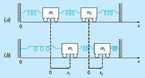
Example: Link the eigenvalue and eigenvector to the characteristic of the given system.
Given stiffness , k = k 1 = k 2 = 200 N/m k = k_1 = k_2 = 200\text{ N/m} k = k 1 = k 2 = 200 N/m
mass , m = m 1 = m 2 = 40 kg m = m_1 = m_2 = 40\text{ kg} m = m 1 = m 2 = 40 kg
The equations of motion of the 2 mass spring systems are provided:
− k x 1 − k ( x 1 − x 2 ) = m 1 x ¨ 1 -kx_1 - k(x_1 - x_2) = m_1\ddot{x}_1 − k x 1 − k ( x 1 − x 2 ) = m 1 x ¨ 1 k ( x 1 − x 2 ) − k x 2 = m 2 x ¨ 2 k(x_1 - x_2) - kx_2 = m_2\ddot{x}_2 k ( x 1 − x 2 ) − k x 2 = m 2 x ¨ 2 where x 1 = A 1 sin ( ω t + θ 1 ) , x ¨ 1 = − ω 2 x 1 \text{where } x_1 = A_1\sin(\omega t + \theta_1) \ , \quad \ddot{x}_1 = -\omega^2x_1 where x 1 = A 1 sin ( ω t + θ 1 ) , x ¨ 1 = − ω 2 x 1 x 2 = A 2 sin ( ω t + θ 2 ) , x ¨ 2 = − ω 2 x 2 x_2 = A_2\sin(\omega t + \theta_2) \ , \quad \ddot{x}_2 = -\omega^2x_2 x 2 = A 2 sin ( ω t + θ 2 ) , x ¨ 2 = − ω 2 x 2
[ 2 k m 1 − ω 2 − k m 1 − k m 2 2 k m 2 − ω 2 ] { x 1 x 2 } = { 0 0 } \begin{bmatrix} \dfrac{2k}{m_1} - \omega^2 & -\dfrac{k}{m_1} \\ -\dfrac{k}{m_2} & \dfrac{2k}{m_2} - \omega^2 \end{bmatrix}\begin{Bmatrix} x_1 \\ x_2 \end{Bmatrix} = \begin{Bmatrix} 0 \\ 0 \end{Bmatrix} m 1 2 k − ω 2 − m 2 k − m 1 k m 2 2 k − ω 2 { x 1 x 2 } = { 0 0 }
Note: The derivation of the eqns involves theory of vibration, thus it is not examined in this study.
[ 10 − ω 2 − 5 − 5 10 − ω 2 ] { x 1 x 2 } = { 0 0 } \begin{bmatrix} 10 - \omega^2 & -5 \\ -5 & 10 - \omega^2 \end{bmatrix}\begin{Bmatrix} x_1 \\ x_2 \end{Bmatrix} = \begin{Bmatrix} 0 \\ 0 \end{Bmatrix} [ 10 − ω 2 − 5 − 5 10 − ω 2 ] { x 1 x 2 } = { 0 0 }
( [ 10 − 5 − 5 10 ] − ω 2 [ 1 0 0 1 ] ) { x 1 x 2 } = { 0 0 } \left(\begin{bmatrix} 10 & -5 \\ -5 & 10 \end{bmatrix} - \omega^2\begin{bmatrix} 1 & 0 \\ 0 & 1 \end{bmatrix}\right)\begin{Bmatrix} x_1 \\ x_2 \end{Bmatrix} = \begin{Bmatrix} 0 \\ 0 \end{Bmatrix} ( [ 10 − 5 − 5 10 ] − ω 2 [ 1 0 0 1 ] ) { x 1 x 2 } = { 0 0 }
[ 10 − 5 − 5 10 ] { x 1 x 2 } − ω 2 { x 1 x 2 } = { 0 0 } \begin{bmatrix} 10 & -5 \\ -5 & 10 \end{bmatrix}\begin{Bmatrix} x_1 \\ x_2 \end{Bmatrix} - \omega^2\begin{Bmatrix} x_1 \\ x_2 \end{Bmatrix} = \begin{Bmatrix} 0 \\ 0 \end{Bmatrix} [ 10 − 5 − 5 10 ] { x 1 x 2 } − ω 2 { x 1 x 2 } = { 0 0 }
[ 10 − 5 − 5 10 ] { x 1 x 2 } = ω 2 { x 1 x 2 } \begin{bmatrix} 10 & -5 \\ -5 & 10 \end{bmatrix}\begin{Bmatrix} x_1 \\ x_2 \end{Bmatrix} = \omega^2\begin{Bmatrix} x_1 \\ x_2 \end{Bmatrix} [ 10 − 5 − 5 10 ] { x 1 x 2 } = ω 2 { x 1 x 2 }
( [ A ] − λ i [ I ] ) { x } i = { 0 } ([A] - \lambda_i[I])\{x\}_i = \{0\} ([ A ] − λ i [ I ]) { x } i = { 0 }
[ A 11 − λ m o d e i A 12 A 21 A 22 − λ m o d e i ] { x 1 x 2 } m o d e i = { 0 0 } \begin{bmatrix} A_{11} - \lambda_{mode\ i} & A_{12} \\ A_{21} & A_{22} - \lambda_{mode\ i} \end{bmatrix}\begin{Bmatrix} x_1 \\ x_2 \end{Bmatrix}_{mode\ i} = \begin{Bmatrix} 0 \\ 0 \end{Bmatrix} [ A 11 − λ m o d e i A 21 A 12 A 22 − λ m o d e i ] { x 1 x 2 } m o d e i = { 0 0 }
( [ A 11 A 12 A 21 A 22 ] − λ m o d e i [ 1 0 0 1 ] ) { x 1 x 2 } m o d e i = { 0 0 } \left(\begin{bmatrix} A_{11} & A_{12} \\ A_{21} & A_{22} \end{bmatrix} - \lambda_{mode\ i}\begin{bmatrix} 1 & 0 \\ 0 & 1 \end{bmatrix}\right)\begin{Bmatrix} x_1 \\ x_2 \end{Bmatrix}_{mode\ i} = \begin{Bmatrix} 0 \\ 0 \end{Bmatrix} ( [ A 11 A 21 A 12 A 22 ] − λ m o d e i [ 1 0 0 1 ] ) { x 1 x 2 } m o d e i = { 0 0 }
[ A 11 A 12 A 21 A 22 ] { x 1 x 2 } m o d e i − λ m o d e i { x 1 x 2 } m o d e i = { 0 0 } \begin{bmatrix} A_{11} & A_{12} \\ A_{21} & A_{22} \end{bmatrix}\begin{Bmatrix} x_1 \\ x_2 \end{Bmatrix}_{mode\ i} - \lambda_{mode\ i}\begin{Bmatrix} x_1 \\ x_2 \end{Bmatrix}_{mode\ i} = \begin{Bmatrix} 0 \\ 0 \end{Bmatrix} [ A 11 A 21 A 12 A 22 ] { x 1 x 2 } m o d e i − λ m o d e i { x 1 x 2 } m o d e i = { 0 0 }
[ A 11 A 12 A 21 A 22 ] { x 1 x 2 } m o d e i = λ m o d e i { x 1 x 2 } m o d e i \begin{bmatrix} A_{11} & A_{12} \\ A_{21} & A_{22} \end{bmatrix}\begin{Bmatrix} x_1 \\ x_2 \end{Bmatrix}_{mode\ i} = \lambda_{mode\ i}\begin{Bmatrix} x_1 \\ x_2 \end{Bmatrix}_{mode\ i} [ A 11 A 21 A 12 A 22 ] { x 1 x 2 } m o d e i = λ m o d e i { x 1 x 2 } m o d e i
By comparing the general formulation of the eigenvalue/eigenvector problem,
[ A ] { x } i = [ λ i ] { x } i [A]\{x\}_i = [\lambda_i]\{x\}_i [ A ] { x } i = [ λ i ] { x } i
We find that the coefficient matrix, [ A ] = [ 10 − 5 − 5 10 ] [A] = \begin{bmatrix} 10 & -5 \\ -5 & 10 \end{bmatrix} [ A ] = [ 10 − 5 − 5 10 ]
Eigenvalue, [ λ i ] = ω 2 [\lambda_i] = \omega^2 [ λ i ] = ω 2 ω \omega ω
Eigenvector, { x } i = { x 1 x 2 } \{x\}_i = \begin{Bmatrix} x_1 \\ x_2 \end{Bmatrix} { x } i = { x 1 x 2 } i i i
Note: Natural frequency and mode shape are important characteristics for a vibration system that can be obtained from the eigenvalue/eigenvector problem.
Example: Solving the eigenvalue/eigenvector problem.
[ 10 − ω 2 − 5 − 5 10 − ω 2 ] { x 1 x 2 } = { 0 0 } \begin{bmatrix} 10 - \omega^2 & -5 \\ -5 & 10 - \omega^2 \end{bmatrix}\begin{Bmatrix} x_1 \\ x_2 \end{Bmatrix} = \begin{Bmatrix} 0 \\ 0 \end{Bmatrix} [ 10 − ω 2 − 5 − 5 10 − ω 2 ] { x 1 x 2 } = { 0 0 }
To have non-trivial solution, { x 1 x 2 } ≠ { 0 0 } \begin{Bmatrix} x_1 \\ x_2 \end{Bmatrix} \neq \begin{Bmatrix} 0 \\ 0 \end{Bmatrix} { x 1 x 2 } = { 0 0 }
∣ 10 − ω 2 − 5 − 5 10 − ω 2 ∣ = 0 \begin{vmatrix} 10 - \omega^2 & -5 \\ -5 & 10 - \omega^2 \end{vmatrix} = 0 10 − ω 2 − 5 − 5 10 − ω 2 = 0
Let the eigenvalue, λ = ω 2 \lambda = \omega^2 λ = ω 2
∣ 10 − λ − 5 − 5 10 − λ ∣ = 0 \begin{vmatrix} 10 - \lambda & -5 \\ -5 & 10 - \lambda \end{vmatrix} = 0 10 − λ − 5 − 5 10 − λ = 0
λ 2 − 20 λ + 75 = 0 Note: This is known as characteristic equation . \lambda^2 - 20\lambda + 75 = 0 \qquad \text{Note: This is known as } \textbf{characteristic equation}. λ 2 − 20 λ + 75 = 0 Note: This is known as characteristic equation .
We obtain 2 eigenvalues for the 2 mass spring system: λ 1 = 5 \lambda_1 = 5 λ 1 = 5 λ 2 = 15 \lambda_2 = 15 λ 2 = 15
Hint: Common practice is to arrange λ i \lambda_i λ i λ 1 < λ 2 \lambda_1 < \lambda_2 λ 1 < λ 2
Since λ = ω 2 \lambda = \omega^2 λ = ω 2 ω 1 = 5 \omega_1 = \sqrt{5} ω 1 = 5 ω 2 = 15 \omega_2 = \sqrt{15} ω 2 = 15
At mode 1, ω 1 = 5 \omega_1 = \sqrt{5} ω 1 = 5 λ 1 = 5 \lambda_1 = 5 λ 1 = 5
[ 5 − 5 − 5 5 ] { x 1 x 2 } 1 = { 0 0 } → expand 5 x 1 − 5 x 2 = 0 − 5 x 1 + 5 x 2 = 0 → x 1 = 1 , x 2 = 1 for both eqns { x 1 x 2 } 1 = { 1 1 } \begin{bmatrix} 5 & -5 \\ -5 & 5 \end{bmatrix}\begin{Bmatrix} x_1 \\ x_2 \end{Bmatrix}_1 = \begin{Bmatrix} 0 \\ 0 \end{Bmatrix} \quad \xrightarrow{\text{expand}} \quad \begin{gathered} 5x_1 - 5x_2 = 0 \\ -5x_1 + 5x_2 = 0 \end{gathered} \quad \xrightarrow{x_1 = 1,\ x_2 = 1 \text{ for both eqns}} \quad \begin{Bmatrix} x_1 \\ x_2 \end{Bmatrix}_1 = \begin{Bmatrix} 1 \\ 1 \end{Bmatrix} [ 5 − 5 − 5 5 ] { x 1 x 2 } 1 = { 0 0 } expand 5 x 1 − 5 x 2 = 0 − 5 x 1 + 5 x 2 = 0 x 1 = 1 , x 2 = 1 for both eqns { x 1 x 2 } 1 = { 1 1 }
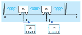
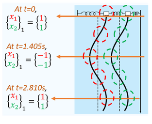
Unscaled eigenvector for mode #1 at ω 1 = 5 \omega_1 = \sqrt{5} ω 1 = 5
{ x 1 x 2 } 1 = { 1 1 } \begin{Bmatrix} x_1 \\ x_2 \end{Bmatrix}_1 = \begin{Bmatrix} 1 \\ 1 \end{Bmatrix} { x 1 x 2 } 1 = { 1 1 } x 1 x_1 x 1 x 2 x_2 x 2
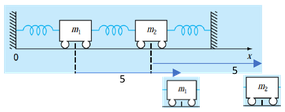
Unscaled eigenvector for mode #1 at ω 1 = 5 \omega_1 = \sqrt{5} ω 1 = 5
{ x 1 x 2 } 1 = { 5 5 } \begin{Bmatrix} x_1 \\ x_2 \end{Bmatrix}_1 = \begin{Bmatrix} 5 \\ 5 \end{Bmatrix} { x 1 x 2 } 1 = { 5 5 } eigenspace , i.e. { x 1 x 2 } 1 = t { 1 1 } \begin{Bmatrix} x_1 \\ x_2 \end{Bmatrix}_1 = t\begin{Bmatrix} 1 \\ 1 \end{Bmatrix} { x 1 x 2 } 1 = t { 1 1 } − ∞ ≤ t ≤ ∞ -\infty \leq t \leq \infty − ∞ ≤ t ≤ ∞
Normalized eigenvector has unique shape and unique scale by using the following formula:
{ x 1 , s c a l e x 2 , s c a l e } 1 = 1 magnitude { x 1 , u n s c a l e x 2 , u n s c a l e } 1 = ± 1 1 2 + 1 2 { 1 1 } = ± 1 5 2 + 5 2 { 5 5 } = ± { 0.707 0.707 } \begin{Bmatrix} x_{1,scale} \\ x_{2,scale} \end{Bmatrix}_1 = \frac{1}{\text{magnitude}\begin{Bmatrix} x_{1,unscale} \\ x_{2,unscale} \end{Bmatrix}_1} = \pm\frac{1}{\sqrt{1^2 + 1^2}}\begin{Bmatrix} 1 \\ 1 \end{Bmatrix} = \pm\frac{1}{\sqrt{5^2 + 5^2}}\begin{Bmatrix} 5 \\ 5 \end{Bmatrix} = \pm\begin{Bmatrix} 0.707 \\ 0.707 \end{Bmatrix} { x 1 , sc a l e x 2 , sc a l e } 1 = magnitude { x 1 , u n sc a l e x 2 , u n sc a l e } 1 1 = ± 1 2 + 1 2 1 { 1 1 } = ± 5 2 + 5 2 1 { 5 5 } = ± { 0.707 0.707 }
At mode 2, ω 2 = 15 \omega_2 = \sqrt{15} ω 2 = 15 λ 2 = 15 \lambda_2 = 15 λ 2 = 15
[ − 5 − 5 − 5 − 5 ] { x 1 x 2 } 2 = { 0 0 } → expand − 5 x 1 − 5 x 2 = 0 − 5 x 1 − 5 x 2 = 0 → x 1 = 1 , x 2 = − 1 for both eqns { x 1 x 2 } 2 = { 1 − 1 } \begin{bmatrix} -5 & -5 \\ -5 & -5 \end{bmatrix}\begin{Bmatrix} x_1 \\ x_2 \end{Bmatrix}_2 = \begin{Bmatrix} 0 \\ 0 \end{Bmatrix} \quad \xrightarrow{\text{expand}} \quad \begin{gathered} -5x_1 - 5x_2 = 0 \\ -5x_1 - 5x_2 = 0 \end{gathered} \quad \xrightarrow{x_1 = 1,\ x_2 = -1 \text{ for both eqns}} \quad \begin{Bmatrix} x_1 \\ x_2 \end{Bmatrix}_2 = \begin{Bmatrix} 1 \\ -1 \end{Bmatrix} [ − 5 − 5 − 5 − 5 ] { x 1 x 2 } 2 = { 0 0 } expand − 5 x 1 − 5 x 2 = 0 − 5 x 1 − 5 x 2 = 0 x 1 = 1 , x 2 = − 1 for both eqns { x 1 x 2 } 2 = { 1 − 1 }
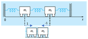
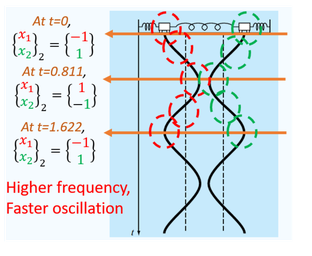
Unscaled eigenvector for mode #2 at ω 2 = 15 \omega_2 = \sqrt{15} ω 2 = 15
{ x 1 x 2 } 2 = { 1 − 1 } \begin{Bmatrix} x_1 \\ x_2 \end{Bmatrix}_2 = \begin{Bmatrix} 1 \\ -1 \end{Bmatrix} { x 1 x 2 } 2 = { 1 − 1 } ω 2 = 15 r a d s − 1 \omega_2 = \sqrt{15}\ rad\,s^{-1} ω 2 = 15 r a d s − 1 x 1 x_1 x 1 x 2 x_2 x 2
Eigenspace for mode #2
{ x 1 x 2 } 2 = t { 1 − 1 } , where − ∞ ≤ t ≤ ∞ . \begin{Bmatrix} x_1 \\ x_2 \end{Bmatrix}_2 = t\begin{Bmatrix} 1 \\ -1 \end{Bmatrix} \ , \text{ where } -\infty \leq t \leq \infty. { x 1 x 2 } 2 = t { 1 − 1 } , where − ∞ ≤ t ≤ ∞.
Normalized eigenvector for mode #2
{ x 1 , s c a l e x 2 , s c a l e } 2 = 1 magnitude { x 1 , u n s c a l e x 2 , u n s c a l e } 2 = ± 1 1 2 + 1 2 { 1 − 1 } = ± { 0.707 − 0.707 } \begin{Bmatrix} x_{1,scale} \\ x_{2,scale} \end{Bmatrix}_2 = \frac{1}{\text{magnitude}\begin{Bmatrix} x_{1,unscale} \\ x_{2,unscale} \end{Bmatrix}_2} = \pm\frac{1}{\sqrt{1^2 + 1^2}}\begin{Bmatrix} 1 \\ -1 \end{Bmatrix} = \pm\begin{Bmatrix} 0.707 \\ -0.707 \end{Bmatrix} { x 1 , sc a l e x 2 , sc a l e } 2 = magnitude { x 1 , u n sc a l e x 2 , u n sc a l e } 2 1 = ± 1 2 + 1 2 1 { 1 − 1 } = ± { 0.707 − 0.707 }
Note: Depending on questions, student should know how to find unscaled eigenvector/ eigenspace/ normalized eigenvector. In general, if it is not stated for manual calculation , then providing unscaled eigenvector (t = 1 t = 1 t = 1 software calculation , normalised eigenvector is used usually.
Visualisation of the eigenvalue & eigenvector information:
Mode 1/ Case 1 Mode 2/ Case 2 Eigenvalue, λ 1 = 5 \lambda_1 = 5 λ 1 = 5 ω 1 = 5 \omega_1 = \sqrt{5} ω 1 = 5 { x 1 x 2 } 1 = ± { 1 1 } \begin{Bmatrix} x_1 \\ x_2 \end{Bmatrix}_1 = \pm\begin{Bmatrix} 1 \\ 1 \end{Bmatrix} { x 1 x 2 } 1 = ± { 1 1 } λ 2 = 15 \lambda_2 = 15 λ 2 = 15 ω 2 = 15 \omega_2 = \sqrt{15} ω 2 = 15 { x 1 x 2 } 2 = ± { 1 − 1 } \begin{Bmatrix} x_1 \\ x_2 \end{Bmatrix}_2 = \pm\begin{Bmatrix} 1 \\ -1 \end{Bmatrix} { x 1 x 2 } 2 = ± { 1 − 1 }
Hint: Period = 1/ Frequency = 2 π / ω 2\pi/\omega 2 π / ω
Example: Find the eigenvalues & eigenvectors of the following matrix.
A = [ 1 − 3 3 3 − 5 3 6 − 6 4 ] \mathbf{A} = \begin{bmatrix} 1 & -3 & 3 \\ 3 & -5 & 3 \\ 6 & -6 & 4 \end{bmatrix} A = 1 3 6 − 3 − 5 − 6 3 3 4
Eigenvalues/eigenvectors problem: ( A − λ I ) x = 0 \qquad (\mathbf{A} - \lambda\mathbf{I})\boldsymbol{x} = \mathbf{0} ( A − λ I ) x = 0
( [ 1 − 3 3 3 − 5 3 6 − 6 4 ] − λ [ 1 0 0 0 1 0 0 0 1 ] ) { x 1 x 2 x 3 } = { 0 0 0 } \left(\begin{bmatrix} 1 & -3 & 3 \\ 3 & -5 & 3 \\ 6 & -6 & 4 \end{bmatrix} - \lambda\begin{bmatrix} 1 & 0 & 0 \\ 0 & 1 & 0 \\ 0 & 0 & 1 \end{bmatrix}\right)\begin{Bmatrix} x_1 \\ x_2 \\ x_3 \end{Bmatrix} = \begin{Bmatrix} 0 \\ 0 \\ 0 \end{Bmatrix} 1 3 6 − 3 − 5 − 6 3 3 4 − λ 1 0 0 0 1 0 0 0 1 ⎩ ⎨ ⎧ x 1 x 2 x 3 ⎭ ⎬ ⎫ = ⎩ ⎨ ⎧ 0 0 0 ⎭ ⎬ ⎫
[ 1 − λ − 3 3 3 − 5 − λ 3 6 − 6 4 − λ ] { x 1 x 2 x 3 } = { 0 0 0 } \begin{bmatrix} 1 - \lambda & -3 & 3 \\ 3 & -5 - \lambda & 3 \\ 6 & -6 & 4 - \lambda \end{bmatrix}\begin{Bmatrix} x_1 \\ x_2 \\ x_3 \end{Bmatrix} = \begin{Bmatrix} 0 \\ 0 \\ 0 \end{Bmatrix} 1 − λ 3 6 − 3 − 5 − λ − 6 3 3 4 − λ ⎩ ⎨ ⎧ x 1 x 2 x 3 ⎭ ⎬ ⎫ = ⎩ ⎨ ⎧ 0 0 0 ⎭ ⎬ ⎫
Since { x 1 x 2 x 3 } ≠ { 0 0 0 } \begin{Bmatrix} x_1 \\ x_2 \\ x_3 \end{Bmatrix} \neq \begin{Bmatrix} 0 \\ 0 \\ 0 \end{Bmatrix} ⎩ ⎨ ⎧ x 1 x 2 x 3 ⎭ ⎬ ⎫ = ⎩ ⎨ ⎧ 0 0 0 ⎭ ⎬ ⎫ ∣ 1 − λ − 3 3 3 − 5 − λ 3 6 − 6 4 − λ ∣ = 0 \qquad \begin{vmatrix} 1 - \lambda & -3 & 3 \\ 3 & -5 - \lambda & 3 \\ 6 & -6 & 4 - \lambda \end{vmatrix} = 0 1 − λ 3 6 − 3 − 5 − λ − 6 3 3 4 − λ = 0
( 1 − λ ) [ ( − 5 − λ ) ( 4 − λ ) − 3 ( − 6 ) ] − ( − 3 ) [ 3 ( 4 − λ ) − 3 ( 6 ) ] + 3 [ 3 ( − 6 ) − ( − 5 − λ ) ( 6 ) ] = 0 (1 - \lambda)\left[(-5 - \lambda)(4 - \lambda) - 3(-6)\right] - (-3)\left[3(4 - \lambda) - 3(6)\right] + 3\left[3(-6) - (-5 - \lambda)(6)\right] = 0 ( 1 − λ ) [ ( − 5 − λ ) ( 4 − λ ) − 3 ( − 6 ) ] − ( − 3 ) [ 3 ( 4 − λ ) − 3 ( 6 ) ] + 3 [ 3 ( − 6 ) − ( − 5 − λ ) ( 6 ) ] = 0
Characteristic eqn: λ 3 − 12 λ − 16 = 0 \qquad \lambda^3 - 12\lambda - 16 = 0 λ 3 − 12 λ − 16 = 0
( λ − 4 ) ( λ 2 + 4 λ + 4 ) = 0 (\lambda - 4)(\lambda^2 + 4\lambda + 4) = 0 ( λ − 4 ) ( λ 2 + 4 λ + 4 ) = 0
λ 1 = − 2 , λ 2 = − 2 (Repeated eigenvalue case) , λ 3 = 4 \lambda_1 = -2 \ , \lambda_2 = -2 \text{ (Repeated eigenvalue case)}, \lambda_3 = 4 λ 1 = − 2 , λ 2 = − 2 (Repeated eigenvalue case) , λ 3 = 4
Case 1: λ 1 = − 2 \lambda_1 = -2 λ 1 = − 2 λ 2 = − 2 \lambda_2 = -2 λ 2 = − 2
[ 3 − 3 3 3 − 3 3 6 − 6 6 ] { x 1 x 2 x 3 } λ = − 2 = { 0 0 0 } \begin{bmatrix} 3 & -3 & 3 \\ 3 & -3 & 3 \\ 6 & -6 & 6 \end{bmatrix}\begin{Bmatrix} x_1 \\ x_2 \\ x_3 \end{Bmatrix}_{\lambda = -2} = \begin{Bmatrix} 0 \\ 0 \\ 0 \end{Bmatrix} 3 3 6 − 3 − 3 − 6 3 3 6 ⎩ ⎨ ⎧ x 1 x 2 x 3 ⎭ ⎬ ⎫ λ = − 2 = ⎩ ⎨ ⎧ 0 0 0 ⎭ ⎬ ⎫
→ augmented [ 1 − 1 1 0 3 − 3 3 0 6 − 6 6 0 ] \xrightarrow{\text{augmented}} \left[\begin{array}{ccc|c} 1 & -1 & 1 & 0 \\ 3 & -3 & 3 & 0 \\ 6 & -6 & 6 & 0 \end{array}\right] augmented 1 3 6 − 1 − 3 − 6 1 3 6 0 0 0
→ R 1 → R 1 3 scale pivot element to 1 [ 1 − 1 1 0 3 − 3 3 0 6 − 6 6 0 ] \xrightarrow[R_1 \to \frac{R_1}{3}]{\text{scale pivot element to 1}} \left[\begin{array}{ccc|c} 1 & -1 & 1 & 0 \\ 3 & -3 & 3 & 0 \\ 6 & -6 & 6 & 0 \end{array}\right] scale pivot element to 1 R 1 → 3 R 1 1 3 6 − 1 − 3 − 6 1 3 6 0 0 0
→ R 2 → R 2 − 3 R 1 , R 3 → R 3 − 6 R 1 Forward elimination [ 1 − 1 1 0 0 0 0 0 0 0 0 0 ] Note: RREF shows rank 1 (i.e. 1 linearly independent vector) \xrightarrow[R_2 \to R_2 - 3R_1,\ R_3 \to R_3 - 6R_1]{\text{Forward elimination}} \left[\begin{array}{ccc|c} 1 & -1 & 1 & 0 \\ 0 & 0 & 0 & 0 \\ 0 & 0 & 0 & 0 \end{array}\right] \qquad \text{Note: RREF shows rank 1 (i.e. 1 linearly independent vector)} Forward elimination R 2 → R 2 − 3 R 1 , R 3 → R 3 − 6 R 1 1 0 0 − 1 0 0 1 0 0 0 0 0 Note: RREF shows rank 1 (i.e. 1 linearly independent vector)
x 1 − x 2 + x 3 = 0 x_1 - x_2 + x_3 = 0 x 1 − x 2 + x 3 = 0
x 1 = x 2 − x 3 x_1 = x_2 - x_3 x 1 = x 2 − x 3
Eigenspace for { x 1 x 2 x 3 } λ = − 2 = { x 2 − x 3 x 2 x 3 } = { x 2 x 2 0 } + { − x 3 0 x 3 } = t { 1 1 0 } ∣ x 2 = t + s { − 1 0 1 } ∣ x 3 = s , where t & s ∈ R \textit{Eigenspace for } \begin{Bmatrix} x_1 \\ x_2 \\ x_3 \end{Bmatrix}_{\lambda = -2} = \begin{Bmatrix} x_2 - x_3 \\ x_2 \\ x_3 \end{Bmatrix} = \begin{Bmatrix} x_2 \\ x_2 \\ 0 \end{Bmatrix} + \begin{Bmatrix} -x_3 \\ 0 \\ x_3 \end{Bmatrix} = t\begin{Bmatrix} 1 \\ 1 \\ 0 \end{Bmatrix}\Bigg|_{x_2 = t} + s\begin{Bmatrix} -1 \\ 0 \\ 1 \end{Bmatrix}\Bigg|_{x_3 = s} \ , \text{where } t \ \& \ s \in \mathbf{R} Eigenspace for ⎩ ⎨ ⎧ x 1 x 2 x 3 ⎭ ⎬ ⎫ λ = − 2 = ⎩ ⎨ ⎧ x 2 − x 3 x 2 x 3 ⎭ ⎬ ⎫ = ⎩ ⎨ ⎧ x 2 x 2 0 ⎭ ⎬ ⎫ + ⎩ ⎨ ⎧ − x 3 0 x 3 ⎭ ⎬ ⎫ = t ⎩ ⎨ ⎧ 1 1 0 ⎭ ⎬ ⎫ x 2 = t + s ⎩ ⎨ ⎧ − 1 0 1 ⎭ ⎬ ⎫ x 3 = s , where t & s ∈ R
Eigenvectors, { x 1 x 2 x 3 } λ = − 2 = { 1 1 0 } & { − 1 0 1 } for repeated eigenvalues λ 1 = − 2 , λ 2 = − 2 respectively. \textit{Eigenvectors, } \begin{Bmatrix} x_1 \\ x_2 \\ x_3 \end{Bmatrix}_{\lambda = -2} = \begin{Bmatrix} 1 \\ 1 \\ 0 \end{Bmatrix} \ \& \ \begin{Bmatrix} -1 \\ 0 \\ 1 \end{Bmatrix} \text{ for repeated eigenvalues } \lambda_1 = -2 \ , \lambda_2 = -2 \text{ respectively.} Eigenvectors, ⎩ ⎨ ⎧ x 1 x 2 x 3 ⎭ ⎬ ⎫ λ = − 2 = ⎩ ⎨ ⎧ 1 1 0 ⎭ ⎬ ⎫ & ⎩ ⎨ ⎧ − 1 0 1 ⎭ ⎬ ⎫ for repeated eigenvalues λ 1 = − 2 , λ 2 = − 2 respectively.
Case 3: λ 3 = 4 \lambda_3 = 4 λ 3 = 4
[ − 3 − 3 3 3 − 9 3 6 − 6 0 ] { x 1 x 2 x 3 } λ = 4 = { 0 0 0 } \begin{bmatrix} -3 & -3 & 3 \\ 3 & -9 & 3 \\ 6 & -6 & 0 \end{bmatrix}\begin{Bmatrix} x_1 \\ x_2 \\ x_3 \end{Bmatrix}_{\lambda = 4} = \begin{Bmatrix} 0 \\ 0 \\ 0 \end{Bmatrix} − 3 3 6 − 3 − 9 − 6 3 3 0 ⎩ ⎨ ⎧ x 1 x 2 x 3 ⎭ ⎬ ⎫ λ = 4 = ⎩ ⎨ ⎧ 0 0 0 ⎭ ⎬ ⎫
→ augmented [ − 3 − 3 3 0 3 − 9 3 0 6 − 6 0 0 ] \xrightarrow{\text{augmented}} \left[\begin{array}{ccc|c} -3 & -3 & 3 & 0 \\ 3 & -9 & 3 & 0 \\ 6 & -6 & 0 & 0 \end{array}\right] augmented − 3 3 6 − 3 − 9 − 6 3 3 0 0 0 0
→ R 1 → − R 1 3 scale pivot element to 1 [ 1 1 − 1 0 3 − 9 3 0 6 − 6 0 0 ] \xrightarrow[R_1 \to -\frac{R_1}{3}]{\text{scale pivot element to 1}} \left[\begin{array}{ccc|c} 1 & 1 & -1 & 0 \\ 3 & -9 & 3 & 0 \\ 6 & -6 & 0 & 0 \end{array}\right] scale pivot element to 1 R 1 → − 3 R 1 1 3 6 1 − 9 − 6 − 1 3 0 0 0 0
→ R 2 → R 2 − 3 R 1 , R 3 → R 3 − 6 R 1 Forward elimination [ 1 1 − 1 0 0 − 12 6 0 0 − 12 6 0 ] \xrightarrow[R_2 \to R_2 - 3R_1,\ R_3 \to R_3 - 6R_1]{\text{Forward elimination}} \left[\begin{array}{ccc|c} 1 & 1 & -1 & 0 \\ 0 & -12 & 6 & 0 \\ 0 & -12 & 6 & 0 \end{array}\right] Forward elimination R 2 → R 2 − 3 R 1 , R 3 → R 3 − 6 R 1 1 0 0 1 − 12 − 12 − 1 6 6 0 0 0
→ R 2 → − R 2 12 scale pivot element to 1 [ 1 1 − 1 0 0 1 − 1 2 0 0 − 12 6 0 ] \xrightarrow[R_2 \to -\frac{R_2}{12}]{\text{scale pivot element to 1}} \left[\begin{array}{ccc|c} 1 & 1 & -1 & 0 \\ 0 & 1 & -\frac{1}{2} & 0 \\ 0 & -12 & 6 & 0 \end{array}\right] scale pivot element to 1 R 2 → − 12 R 2 1 0 0 1 1 − 12 − 1 − 2 1 6 0 0 0
→ R 3 → R 3 + 12 R 2 Forward elimination [ 1 1 − 1 0 0 1 − 1 2 0 0 0 0 0 ] \xrightarrow[R_3 \to R_3 + 12R_2]{\text{Forward elimination}} \left[\begin{array}{ccc|c} 1 & 1 & -1 & 0 \\ 0 & 1 & -\frac{1}{2} & 0 \\ 0 & 0 & 0 & 0 \end{array}\right] Forward elimination R 3 → R 3 + 12 R 2 1 0 0 1 1 0 − 1 − 2 1 0 0 0 0
→ R 1 → R 1 − R 2 Forward elimination [ 1 0 − 1 2 0 0 1 − 1 2 0 0 0 0 0 ] Note: RREF shows rank 2 (i.e. 2 linearly independent vectors) \xrightarrow[R_1 \to R_1 - R_2]{\text{Forward elimination}} \left[\begin{array}{ccc|c} 1 & 0 & -\frac{1}{2} & 0 \\ 0 & 1 & -\frac{1}{2} & 0 \\ 0 & 0 & 0 & 0 \end{array}\right] \qquad \text{Note: RREF shows rank 2 (i.e. 2 linearly independent vectors)} Forward elimination R 1 → R 1 − R 2 1 0 0 0 1 0 − 2 1 − 2 1 0 0 0 0 Note: RREF shows rank 2 (i.e. 2 linearly independent vectors)
x 1 − 1 2 x 3 = 0 > > x 1 = 1 2 x 3 x_1 - \frac{1}{2}x_3 = 0 \quad >> \quad x_1 = \frac{1}{2}x_3 x 1 − 2 1 x 3 = 0 >> x 1 = 2 1 x 3
x 2 − 1 2 x 3 = 0 > > x 2 = 1 2 x 3 x_2 - \frac{1}{2}x_3 = 0 \quad >> \quad x_2 = \frac{1}{2}x_3 x 2 − 2 1 x 3 = 0 >> x 2 = 2 1 x 3
Eigenspace for { x 1 x 2 x 3 } λ = 4 = { 1 2 x 3 1 2 x 3 x 3 } = t { 1 2 1 2 1 } ∣ x 3 = t , where t ∈ R \textit{Eigenspace for } \begin{Bmatrix} x_1 \\ x_2 \\ x_3 \end{Bmatrix}_{\lambda = 4} = \begin{Bmatrix} \frac{1}{2}x_3 \\ \frac{1}{2}x_3 \\ x_3 \end{Bmatrix} = t\begin{Bmatrix} \frac{1}{2} \\ \frac{1}{2} \\ 1 \end{Bmatrix}\Bigg|_{x_3 = t} \ , \text{where } t \in \mathbf{R} Eigenspace for ⎩ ⎨ ⎧ x 1 x 2 x 3 ⎭ ⎬ ⎫ λ = 4 = ⎩ ⎨ ⎧ 2 1 x 3 2 1 x 3 x 3 ⎭ ⎬ ⎫ = t ⎩ ⎨ ⎧ 2 1 2 1 1 ⎭ ⎬ ⎫ x 3 = t , where t ∈ R
Eigenvector, { x 1 x 2 x 3 } λ = 4 = { 0.5 0.5 1 } \textit{Eigenvector, } \begin{Bmatrix} x_1 \\ x_2 \\ x_3 \end{Bmatrix}_{\lambda = 4} = \begin{Bmatrix} 0.5 \\ 0.5 \\ 1 \end{Bmatrix} Eigenvector, ⎩ ⎨ ⎧ x 1 x 2 x 3 ⎭ ⎬ ⎫ λ = 4 = ⎩ ⎨ ⎧ 0.5 0.5 1 ⎭ ⎬ ⎫
For verification of the eigenvector results, it should satisfy the eigenvalue/eigenvector problem:
[ A ] { x } i = [ λ i ] { x } i [A]\{x\}_i = [\lambda_i]\{x\}_i [ A ] { x } i = [ λ i ] { x } i
Case 1 (λ = − 2 \lambda = -2 λ = − 2 Case 2 (λ = − 2 \lambda = -2 λ = − 2 Case 3 (λ = 4 \lambda = 4 λ = 4 [ 1 − 3 3 3 − 5 3 6 − 6 4 ] { 1 1 0 } = − 2 { 1 1 0 } \begin{bmatrix} 1 & -3 & 3 \\ 3 & -5 & 3 \\ 6 & -6 & 4 \end{bmatrix}\begin{Bmatrix} 1 \\ 1 \\ 0 \end{Bmatrix} = -2\begin{Bmatrix} 1 \\ 1 \\ 0 \end{Bmatrix} 1 3 6 − 3 − 5 − 6 3 3 4 ⎩ ⎨ ⎧ 1 1 0 ⎭ ⎬ ⎫ = − 2 ⎩ ⎨ ⎧ 1 1 0 ⎭ ⎬ ⎫ [ 1 − 3 3 3 − 5 3 6 − 6 4 ] { − 1 0 1 } = − 2 { − 1 0 1 } \begin{bmatrix} 1 & -3 & 3 \\ 3 & -5 & 3 \\ 6 & -6 & 4 \end{bmatrix}\begin{Bmatrix} -1 \\ 0 \\ 1 \end{Bmatrix} = -2\begin{Bmatrix} -1 \\ 0 \\ 1 \end{Bmatrix} 1 3 6 − 3 − 5 − 6 3 3 4 ⎩ ⎨ ⎧ − 1 0 1 ⎭ ⎬ ⎫ = − 2 ⎩ ⎨ ⎧ − 1 0 1 ⎭ ⎬ ⎫ [ 1 − 3 3 3 − 5 3 6 − 6 4 ] { 0.5 0.5 1 } = 4 { 0.5 0.5 1 } \begin{bmatrix} 1 & -3 & 3 \\ 3 & -5 & 3 \\ 6 & -6 & 4 \end{bmatrix}\begin{Bmatrix} 0.5 \\ 0.5 \\ 1 \end{Bmatrix} = 4\begin{Bmatrix} 0.5 \\ 0.5 \\ 1 \end{Bmatrix} 1 3 6 − 3 − 5 − 6 3 3 4 ⎩ ⎨ ⎧ 0.5 0.5 1 ⎭ ⎬ ⎫ = 4 ⎩ ⎨ ⎧ 0.5 0.5 1 ⎭ ⎬ ⎫
Or we can combine all cases into single matrix operation:
Eigenvector/ Modal matrix consists of all eigenvectors, P \mathbf{P} P Eigenvalue/ Spectral matrix consists of all eigenvalues, D \mathbf{D} D Verification of Eigenvalue/ Eigenvector Problem for All Cases P \mathbf{P} P [ P ] [P] [ P ] = [ { x 1 x 2 x 3 } 1 { x 1 x 2 x 3 } 2 { x 1 x 2 x 3 } 3 ] = \left[\begin{Bmatrix} x_1 \\ x_2 \\ x_3 \end{Bmatrix}_1 \begin{Bmatrix} x_1 \\ x_2 \\ x_3 \end{Bmatrix}_2 \begin{Bmatrix} x_1 \\ x_2 \\ x_3 \end{Bmatrix}_3\right] = ⎩ ⎨ ⎧ x 1 x 2 x 3 ⎭ ⎬ ⎫ 1 ⎩ ⎨ ⎧ x 1 x 2 x 3 ⎭ ⎬ ⎫ 2 ⎩ ⎨ ⎧ x 1 x 2 x 3 ⎭ ⎬ ⎫ 3 = [ 1 − 1 0.5 1 0 0.5 0 1 1 ] = \begin{bmatrix} 1 & -1 & 0.5 \\ 1 & 0 & 0.5 \\ 0 & 1 & 1 \end{bmatrix} = 1 1 0 − 1 0 1 0.5 0.5 1 { x 1 x 2 x 3 } 1 = eigenvector #1 \begin{Bmatrix} x_1 \\ x_2 \\ x_3 \end{Bmatrix}_1 = \textit{eigenvector \#1} ⎩ ⎨ ⎧ x 1 x 2 x 3 ⎭ ⎬ ⎫ 1 = eigenvector #1 D \mathbf{D} D [ D ] [D] [ D ] = [ λ 1 0 0 0 λ 2 0 0 0 λ 3 ] = \begin{bmatrix} \lambda_1 & 0 & 0 \\ 0 & \lambda_2 & 0 \\ 0 & 0 & \lambda_3 \end{bmatrix} = λ 1 0 0 0 λ 2 0 0 0 λ 3 = [ − 2 0 0 0 − 2 0 0 0 4 ] = \begin{bmatrix} -2 & 0 & 0 \\ 0 & -2 & 0 \\ 0 & 0 & 4 \end{bmatrix} = − 2 0 0 0 − 2 0 0 0 4 λ 1 = eigenvalue #1 \lambda_1 = \textit{eigenvalue \#1} λ 1 = eigenvalue #1 [ A ] { x } i = [ λ i ] { x } i → extend [A]\{x\}_i = [\lambda_i]\{x\}_i \xrightarrow{\text{extend}} [ A ] { x } i = [ λ i ] { x } i extend [ A ] [ P ] = [ P ] [ D ] [A][P] = [P][D] [ A ] [ P ] = [ P ] [ D ] [ 1 − 3 3 3 − 5 3 6 − 6 4 ] [ 1 − 1 0.5 1 0 0.5 0 1 1 ] = [ 1 − 1 0.5 1 0 0.5 0 1 1 ] [ − 2 0 0 0 − 2 0 0 0 4 ] \begin{bmatrix} 1 & -3 & 3 \\ 3 & -5 & 3 \\ 6 & -6 & 4 \end{bmatrix}\begin{bmatrix} 1 & -1 & 0.5 \\ 1 & 0 & 0.5 \\ 0 & 1 & 1 \end{bmatrix} = \begin{bmatrix} 1 & -1 & 0.5 \\ 1 & 0 & 0.5 \\ 0 & 1 & 1 \end{bmatrix}\begin{bmatrix} -2 & 0 & 0 \\ 0 & -2 & 0 \\ 0 & 0 & 4 \end{bmatrix} 1 3 6 − 3 − 5 − 6 3 3 4 1 1 0 − 1 0 1 0.5 0.5 1 = 1 1 0 − 1 0 1 0.5 0.5 1 − 2 0 0 0 − 2 0 0 0 4 = − 2 [ 1 0 0 1 0 0 0 0 0 ] − 2 [ 0 − 1 0 0 0 0 0 1 0 ] + 4 [ 0 0 0.5 0 0 0.5 0 0 1 ] = -2\begin{bmatrix} 1 & 0 & 0 \\ 1 & 0 & 0 \\ 0 & 0 & 0 \end{bmatrix} -2\begin{bmatrix} 0 & -1 & 0 \\ 0 & 0 & 0 \\ 0 & 1 & 0 \end{bmatrix} + 4\begin{bmatrix} 0 & 0 & 0.5 \\ 0 & 0 & 0.5 \\ 0 & 0 & 1 \end{bmatrix} = − 2 1 1 0 0 0 0 0 0 0 − 2 0 0 0 − 1 0 1 0 0 0 + 4 0 0 0 0 0 0 0.5 0.5 1 ∴ \therefore ∴ Since LHS = RHS, [ P ] [P] [ P ] [ D ] [D] [ D ]
7.3 Engineering Application of Eigenvalue/Eigenvector Problem
(a) Diagonalization
Eigenvectors are useful to diagonalize a square matrix:
D = P − 1 A P \mathbf{D} = \mathbf{P}^{-1}\mathbf{A}\mathbf{P} D = P − 1 AP ∣ P ∣ ≠ 0 |\mathbf{P}| \neq 0 ∣ P ∣ = 0 P = \mathbf{P} = P = full rank eigenvector or modal matrix
Previously, eigenvalues/eigenvectors problem: ( A − λ I ) x = 0 \qquad (\mathbf{A} - \lambda\mathbf{I})\boldsymbol{x} = \mathbf{0} ( A − λ I ) x = 0
A = [ 1 − 3 3 3 − 5 3 6 − 6 4 ] → [ 1 − λ − 3 3 3 − 5 − λ 3 6 − 6 4 − λ ] { x 1 x 2 x 3 } = { 0 0 0 } \mathbf{A} = \begin{bmatrix} 1 & -3 & 3 \\ 3 & -5 & 3 \\ 6 & -6 & 4 \end{bmatrix} \rightarrow \begin{bmatrix} 1 - \lambda & -3 & 3 \\ 3 & -5 - \lambda & 3 \\ 6 & -6 & 4 - \lambda \end{bmatrix}\begin{Bmatrix} x_1 \\ x_2 \\ x_3 \end{Bmatrix} = \begin{Bmatrix} 0 \\ 0 \\ 0 \end{Bmatrix} A = 1 3 6 − 3 − 5 − 6 3 3 4 → 1 − λ 3 6 − 3 − 5 − λ − 6 3 3 4 − λ ⎩ ⎨ ⎧ x 1 x 2 x 3 ⎭ ⎬ ⎫ = ⎩ ⎨ ⎧ 0 0 0 ⎭ ⎬ ⎫
Eigenvectors, { x 1 x 2 x 3 } λ = − 2 = { 1 1 0 } & { − 1 0 1 } \textit{Eigenvectors, } \begin{Bmatrix} x_1 \\ x_2 \\ x_3 \end{Bmatrix}_{\lambda = -2} = \begin{Bmatrix} 1 \\ 1 \\ 0 \end{Bmatrix} \ \& \ \begin{Bmatrix} -1 \\ 0 \\ 1 \end{Bmatrix} Eigenvectors, ⎩ ⎨ ⎧ x 1 x 2 x 3 ⎭ ⎬ ⎫ λ = − 2 = ⎩ ⎨ ⎧ 1 1 0 ⎭ ⎬ ⎫ & ⎩ ⎨ ⎧ − 1 0 1 ⎭ ⎬ ⎫
Eigenvector, { x 1 x 2 x 3 } λ = 4 = { 0.5 0.5 1 } \textit{Eigenvector, } \begin{Bmatrix} x_1 \\ x_2 \\ x_3 \end{Bmatrix}_{\lambda = 4} = \begin{Bmatrix} 0.5 \\ 0.5 \\ 1 \end{Bmatrix} Eigenvector, ⎩ ⎨ ⎧ x 1 x 2 x 3 ⎭ ⎬ ⎫ λ = 4 = ⎩ ⎨ ⎧ 0.5 0.5 1 ⎭ ⎬ ⎫
∴ Eigenvector matrix consists of all eigenvectors, P = [ { x 1 x 2 x 3 } λ 1 { x 1 x 2 x 3 } λ 2 { x 1 x 2 x 3 } λ 3 ] = [ 1 − 1 0.5 1 0 0.5 0 1 1 ] \therefore \textit{Eigenvector matrix consists of all eigenvectors, } \mathbf{P} = \left[\begin{Bmatrix} x_1 \\ x_2 \\ x_3 \end{Bmatrix}_{\lambda_1} \begin{Bmatrix} x_1 \\ x_2 \\ x_3 \end{Bmatrix}_{\lambda_2} \begin{Bmatrix} x_1 \\ x_2 \\ x_3 \end{Bmatrix}_{\lambda_3}\right] = \begin{bmatrix} 1 & -1 & 0.5 \\ 1 & 0 & 0.5 \\ 0 & 1 & 1 \end{bmatrix} ∴ Eigenvector matrix consists of all eigenvectors, P = ⎩ ⎨ ⎧ x 1 x 2 x 3 ⎭ ⎬ ⎫ λ 1 ⎩ ⎨ ⎧ x 1 x 2 x 3 ⎭ ⎬ ⎫ λ 2 ⎩ ⎨ ⎧ x 1 x 2 x 3 ⎭ ⎬ ⎫ λ 3 = 1 1 0 − 1 0 1 0.5 0.5 1
D = P − 1 A P = [ 1 − 1 0.5 1 0 0.5 0 1 1 ] − 1 [ 1 − 3 3 3 − 5 3 6 − 6 4 ] [ 1 − 1 0.5 1 0 0.5 0 1 1 ] = [ − 2 0 0 0 − 2 0 0 0 4 ] \mathbf{D} = \mathbf{P}^{-1}\mathbf{A}\mathbf{P} = \begin{bmatrix} 1 & -1 & 0.5 \\ 1 & 0 & 0.5 \\ 0 & 1 & 1 \end{bmatrix}^{-1}\begin{bmatrix} 1 & -3 & 3 \\ 3 & -5 & 3 \\ 6 & -6 & 4 \end{bmatrix}\begin{bmatrix} 1 & -1 & 0.5 \\ 1 & 0 & 0.5 \\ 0 & 1 & 1 \end{bmatrix} = \begin{bmatrix} -2 & 0 & 0 \\ 0 & -2 & 0 \\ 0 & 0 & 4 \end{bmatrix} D = P − 1 AP = 1 1 0 − 1 0 1 0.5 0.5 1 − 1 1 3 6 − 3 − 5 − 6 3 3 4 1 1 0 − 1 0 1 0.5 0.5 1 = − 2 0 0 0 − 2 0 0 0 4
Note: We can convert a non-diagonal matrix A \mathbf{A} A D \mathbf{D} D A \mathbf{A} A λ 1 = − 2 , λ 2 = − 2 , λ 3 = 4 \lambda_1 = -2 \ , \lambda_2 = -2, \lambda_3 = 4 λ 1 = − 2 , λ 2 = − 2 , λ 3 = 4
(b) Extension from Diagonalization
D = P − 1 A P \mathbf{D} = \mathbf{P}^{-1}\mathbf{A}\mathbf{P} D = P − 1 AP
A = P D P − 1 \mathbf{A} = \mathbf{P}\mathbf{D}\mathbf{P}^{-1} A = PD P − 1
,where A \mathbf{A} A P \mathbf{P} P D \mathbf{D} D
A 2 = A A = ( P D P − 1 ) ( P D P − 1 ) = ( P D 2 P − 1 ) where P − 1 P = I \mathbf{A}^2 = \mathbf{A}\mathbf{A} = (\mathbf{P}\mathbf{D}\mathbf{P}^{-1})(\mathbf{P}\mathbf{D}\mathbf{P}^{-1}) = (\mathbf{P}\mathbf{D}^2\mathbf{P}^{-1}) \qquad \text{where } \mathbf{P}^{-1}\mathbf{P} = \mathbf{I} A 2 = AA = ( PD P − 1 ) ( PD P − 1 ) = ( P D 2 P − 1 ) where P − 1 P = I
A 3 = A 2 A = ( P D 2 P − 1 ) ( P D P − 1 ) = ( P D 3 P − 1 ) \mathbf{A}^3 = \mathbf{A}^2\mathbf{A} = (\mathbf{P}\mathbf{D}^2\mathbf{P}^{-1})(\mathbf{P}\mathbf{D}\mathbf{P}^{-1}) = (\mathbf{P}\mathbf{D}^3\mathbf{P}^{-1}) A 3 = A 2 A = ( P D 2 P − 1 ) ( PD P − 1 ) = ( P D 3 P − 1 )
⋮ \vdots ⋮
A k = P D k P − 1 where D k = [ λ 1 0 0 0 λ 2 0 0 0 λ 3 ] k = [ λ 1 k 0 0 0 λ 2 k 0 0 0 λ 3 k ] , where k ∈ R \mathbf{A}^k = \mathbf{P}\mathbf{D}^k\mathbf{P}^{-1} \qquad \text{where } \mathbf{D}^k = \begin{bmatrix} \lambda_1 & 0 & 0 \\ 0 & \lambda_2 & 0 \\ 0 & 0 & \lambda_3 \end{bmatrix}^k = \begin{bmatrix} \lambda_1^k & 0 & 0 \\ 0 & \lambda_2^k & 0 \\ 0 & 0 & \lambda_3^k \end{bmatrix} \ , \text{where } k \in \mathbf{R} A k = P D k P − 1 where D k = λ 1 0 0 0 λ 2 0 0 0 λ 3 k = λ 1 k 0 0 0 λ 2 k 0 0 0 λ 3 k , where k ∈ R
(Comment: power of a diagonal matrix can be computed easily!)
Note: This formula implies that change of power of A \mathbf{A} A A \mathbf{A} A λ 1 , λ 2 , λ 3 \lambda_1, \lambda_2, \lambda_3 λ 1 , λ 2 , λ 3 A k \mathbf{A}^k A k λ 1 k , λ 2 k , λ 3 k \lambda_1^k, \lambda_2^k, \lambda_3^k λ 1 k , λ 2 k , λ 3 k A − 1 \mathbf{A}^{-1} A − 1 1 λ 1 , 1 λ 2 , 1 λ 3 \dfrac{1}{\lambda_1}, \dfrac{1}{\lambda_2}, \dfrac{1}{\lambda_3} λ 1 1 , λ 2 1 , λ 3 1
You can find A k \mathbf{A}^k A k
A = [ 1 − 3 3 3 − 5 3 6 − 6 4 ] ; Eigenvalue matrix, D = [ − 2 0 0 0 − 2 0 0 0 4 ] ; Eigenvector matrix, P = [ 1 − 1 0.5 1 0 0.5 0 1 1 ] \mathbf{A} = \begin{bmatrix} 1 & -3 & 3 \\ 3 & -5 & 3 \\ 6 & -6 & 4 \end{bmatrix} \ ; \quad \text{Eigenvalue matrix, } \mathbf{D} = \begin{bmatrix} -2 & 0 & 0 \\ 0 & -2 & 0 \\ 0 & 0 & 4 \end{bmatrix} ; \quad \text{Eigenvector matrix, } \mathbf{P} = \begin{bmatrix} 1 & -1 & 0.5 \\ 1 & 0 & 0.5 \\ 0 & 1 & 1 \end{bmatrix} A = 1 3 6 − 3 − 5 − 6 3 3 4 ; Eigenvalue matrix, D = − 2 0 0 0 − 2 0 0 0 4 ; Eigenvector matrix, P = 1 1 0 − 1 0 1 0.5 0.5 1
A 100 = P D 100 P − 1 = [ 1 − 1 0.5 1 0 0.5 0 1 1 ] [ − 2 0 0 0 − 2 0 0 0 4 ] 100 [ 1 − 1 0.5 1 0 0.5 0 1 1 ] − 1 = [ 1 − 1 0.5 1 0 0.5 0 1 1 ] [ ( − 2 ) 100 0 0 0 ( − 2 ) 100 0 0 0 ( 4 ) 100 ] [ 1 − 1 0.5 1 0 0.5 0 1 1 ] − 1 = 10 60 × [ 0.8035 − 0.8035 0.8035 0.8035 − 0.8035 0.8035 1.6069 − 1.6069 1.6069 ] \begin{aligned}
\mathbf{A}^{100} = \mathbf{P}\mathbf{D}^{100}\mathbf{P}^{-1} &= \begin{bmatrix} 1 & -1 & 0.5 \\ 1 & 0 & 0.5 \\ 0 & 1 & 1 \end{bmatrix}\begin{bmatrix} -2 & 0 & 0 \\ 0 & -2 & 0 \\ 0 & 0 & 4 \end{bmatrix}^{100}\begin{bmatrix} 1 & -1 & 0.5 \\ 1 & 0 & 0.5 \\ 0 & 1 & 1 \end{bmatrix}^{-1} \\
&= \begin{bmatrix} 1 & -1 & 0.5 \\ 1 & 0 & 0.5 \\ 0 & 1 & 1 \end{bmatrix}\begin{bmatrix} (-2)^{100} & 0 & 0 \\ 0 & (-2)^{100} & 0 \\ 0 & 0 & (4)^{100} \end{bmatrix}\begin{bmatrix} 1 & -1 & 0.5 \\ 1 & 0 & 0.5 \\ 0 & 1 & 1 \end{bmatrix}^{-1} \\
&= 10^{60} \times \begin{bmatrix} 0.8035 & -0.8035 & 0.8035 \\ 0.8035 & -0.8035 & 0.8035 \\ 1.6069 & -1.6069 & 1.6069 \end{bmatrix}
\end{aligned} A 100 = P D 100 P − 1 = 1 1 0 − 1 0 1 0.5 0.5 1 − 2 0 0 0 − 2 0 0 0 4 100 1 1 0 − 1 0 1 0.5 0.5 1 − 1 = 1 1 0 − 1 0 1 0.5 0.5 1 ( − 2 ) 100 0 0 0 ( − 2 ) 100 0 0 0 ( 4 ) 100 1 1 0 − 1 0 1 0.5 0.5 1 − 1 = 1 0 60 × 0.8035 0.8035 1.6069 − 0.8035 − 0.8035 − 1.6069 0.8035 0.8035 1.6069 Some useful properties of eigenvalues,
λ i \lambda_i λ i Trace( A ) = ∑ λ i → 1 − 5 + 4 = − 2 − 2 + 4 = 0 (\mathbf{A}) = \sum\lambda_i \qquad \rightarrow \qquad 1 - 5 + 4 = -2 - 2 + 4 = 0 ( A ) = ∑ λ i → 1 − 5 + 4 = − 2 − 2 + 4 = 0
Determinant( A ) = ∏ λ i → 1 ( − 20 + 18 ) − ( − 3 ) ( 12 − 18 ) + 3 ( − 18 + 30 ) = ( − 2 ) ( − 2 ) ( 4 ) = 16 (\mathbf{A}) = \prod\lambda_i \rightarrow 1(-20 + 18) - (-3)(12 - 18) + 3(-18 + 30) = (-2)(-2)(4) = 16 ( A ) = ∏ λ i → 1 ( − 20 + 18 ) − ( − 3 ) ( 12 − 18 ) + 3 ( − 18 + 30 ) = ( − 2 ) ( − 2 ) ( 4 ) = 16
Eigenvalue ( A ) = (\mathbf{A}) = ( A ) = ( A T ) = λ i → λ 1 = − 2 ; λ 2 = − 2 ; λ 3 = 4 (\mathbf{A}^T) = \lambda_i \qquad \rightarrow \qquad \lambda_1 = -2; \lambda_2 = -2; \lambda_3 = 4 ( A T ) = λ i → λ 1 = − 2 ; λ 2 = − 2 ; λ 3 = 4
Eigenvalue ( k A ) = k λ i (k\mathbf{A}) = k\lambda_i ( k A ) = k λ i k ∈ R → k \in \mathbf{R} \qquad \rightarrow \qquad k ∈ R → ( 5 A ) = 5 λ 1 = − 10 ; 5 λ 2 = − 10 ; 5 λ 3 = 20 (\mathbf{5A}) = 5\lambda_1 = -10; 5\lambda_2 = -10; 5\lambda_3 = 20 ( 5A ) = 5 λ 1 = − 10 ; 5 λ 2 = − 10 ; 5 λ 3 = 20
Eigenvalue ( A k ) = λ i k (\mathbf{A}^k) = \lambda_i^k ( A k ) = λ i k k ∈ R → k \in \mathbf{R} \qquad \rightarrow \qquad k ∈ R → ( A 5 ) = λ 1 5 = ( − 2 ) 5 ; λ 2 5 = ( − 2 ) 5 ; λ 3 5 = ( 4 ) 5 (\mathbf{A}^5) = \lambda_1^5 = (-2)^5; \lambda_2^5 = (-2)^5; \lambda_3^5 = (4)^5 ( A 5 ) = λ 1 5 = ( − 2 ) 5 ; λ 2 5 = ( − 2 ) 5 ; λ 3 5 = ( 4 ) 5
Eigenvalue ( A ± k I ) = λ i ± k → (\mathbf{A} \pm k\mathbf{I}) = \lambda_i \pm k \qquad \rightarrow \qquad ( A ± k I ) = λ i ± k → ( A + 5 I ) = λ 1 + 5 = 3 ; λ 2 + 5 = 3 ; λ 3 + 5 = 9 (\mathbf{A} + 5\mathbf{I}) = \lambda_1 + 5 = 3; \lambda_2 + 5 = 3; \lambda_3 + 5 = 9 ( A + 5 I ) = λ 1 + 5 = 3 ; λ 2 + 5 = 3 ; λ 3 + 5 = 9
(c) Cayley-Hamilton Theorem
Characteristic equation of eigenvalue/eigenvector problem is useful to compute the power of matrix.
Previously, eigenvalues/eigenvectors problem: ( A − λ I ) x = 0 \qquad (\mathbf{A} - \lambda\mathbf{I})\boldsymbol{x} = \mathbf{0} ( A − λ I ) x = 0
A = [ 1 − 3 3 3 − 5 3 6 − 6 4 ] → [ 1 − λ − 3 3 3 − 5 − λ 3 6 − 6 4 − λ ] { x 1 x 2 x 3 } = { 0 0 0 } \mathbf{A} = \begin{bmatrix} 1 & -3 & 3 \\ 3 & -5 & 3 \\ 6 & -6 & 4 \end{bmatrix} \rightarrow \begin{bmatrix} 1 - \lambda & -3 & 3 \\ 3 & -5 - \lambda & 3 \\ 6 & -6 & 4 - \lambda \end{bmatrix}\begin{Bmatrix} x_1 \\ x_2 \\ x_3 \end{Bmatrix} = \begin{Bmatrix} 0 \\ 0 \\ 0 \end{Bmatrix} A = 1 3 6 − 3 − 5 − 6 3 3 4 → 1 − λ 3 6 − 3 − 5 − λ − 6 3 3 4 − λ ⎩ ⎨ ⎧ x 1 x 2 x 3 ⎭ ⎬ ⎫ = ⎩ ⎨ ⎧ 0 0 0 ⎭ ⎬ ⎫
Characteristic eqn: f ( λ ) = ∣ ( A − λ I ) ∣ = 0 f(\lambda) = |(\mathbf{A} - \lambda\mathbf{I})| = 0 f ( λ ) = ∣ ( A − λ I ) ∣ = 0 λ \lambda λ
p 0 + p 1 λ + p 2 λ 2 + ⋯ + p n λ n = 0 p_0 + p_1\lambda + p_2\lambda^2 + \cdots + p_n\lambda^n = 0 p 0 + p 1 λ + p 2 λ 2 + ⋯ + p n λ n = 0
λ 3 − 12 λ − 16 = 0 \lambda^3 - 12\lambda - 16 = 0 λ 3 − 12 λ − 16 = 0
Cayley-Hamilton Theorem: f ( A ) = p 0 I + p 1 A + p 2 A 2 + ⋯ + p n A n = 0 f(\mathbf{A}) = p_0\mathbf{I} + p_1\mathbf{A} + p_2\mathbf{A}^2 + \cdots + p_n\mathbf{A}^n = 0 f ( A ) = p 0 I + p 1 A + p 2 A 2 + ⋯ + p n A n = 0
,where A \mathbf{A} A λ \lambda λ A \mathbf{A} A
A 3 − 12 A − 16 I = 0 [ C a y l e y − H a m i l t o n F o r m ] \mathbf{A}^3 - 12\mathbf{A} - 16\mathbf{I} = \mathbf{0} \qquad [\mathit{Cayley} - \mathit{Hamilton}\ \mathit{Form}] A 3 − 12 A − 16 I = 0 [ Cayley − Hamilton Form ]
You can find A n \mathbf{A}^n A n
A 2 − 12 I − 16 A − 1 = 0 → A − 1 = 1 16 ( A 2 − 12 I ) \mathbf{A}^2 - 12\mathbf{I} - 16\mathbf{A}^{-1} = \mathbf{0} \qquad \rightarrow \qquad \mathbf{A}^{-1} = \frac{1}{16}(\mathbf{A}^2 - 12\mathbf{I}) A 2 − 12 I − 16 A − 1 = 0 → A − 1 = 16 1 ( A 2 − 12 I )
A 3 = 12 A + 16 I \mathbf{A}^3 = 12\mathbf{A} + 16\mathbf{I} A 3 = 12 A + 16 I
A 4 = 12 A 2 + 16 A = 12 ( 12 I + 16 A − 1 ) + 16 A \mathbf{A}^4 = 12\mathbf{A}^2 + 16\mathbf{A} = 12(12\mathbf{I} + 16\mathbf{A}^{-1}) + 16\mathbf{A} A 4 = 12 A 2 + 16 A = 12 ( 12 I + 16 A − 1 ) + 16 A
A 5 = 12 A 3 + 16 A 2 = 12 ( 12 A + 16 I ) + 16 ( 12 I + 16 A − 1 ) \mathbf{A}^5 = 12\mathbf{A}^3 + 16\mathbf{A}^2 = 12(12\mathbf{A} + 16\mathbf{I}) + 16(12\mathbf{I} + 16\mathbf{A}^{-1}) A 5 = 12 A 3 + 16 A 2 = 12 ( 12 A + 16 I ) + 16 ( 12 I + 16 A − 1 )
⋮ \vdots ⋮
7.4 Engineering Application of Solving Homogeneous System of Linear Equations
So far, we have determined the eigenvalue & eigenvector for a homogeneous system of linear equations. This information is useful to find the eigenfunction (i.e. Each of a set of independent functions which are the solutions to a given differential equation.)
Given stiffness , k = k 1 = k 2 = 200 N/m k = k_1 = k_2 = 200\text{ N/m} k = k 1 = k 2 = 200 N/m
mass , m = m 1 = m 2 = 40 kg m = m_1 = m_2 = 40\text{ kg} m = m 1 = m 2 = 40 kg
The equations of motion of the 2 mass spring systems are provided:
− k x 1 − k ( x 1 − x 2 ) = m 1 x ¨ 1 -kx_1 - k(x_1 - x_2) = m_1\ddot{x}_1 − k x 1 − k ( x 1 − x 2 ) = m 1 x ¨ 1 k ( x 1 − x 2 ) − k x 2 = m 2 x ¨ 2 k(x_1 - x_2) - kx_2 = m_2\ddot{x}_2 k ( x 1 − x 2 ) − k x 2 = m 2 x ¨ 2 where x 1 = A 1 sin ( ω t + θ 1 ) , x ¨ 1 = − ω 2 x 1 \text{where } x_1 = A_1\sin(\omega t + \theta_1) \ , \quad \ddot{x}_1 = -\omega^2x_1 where x 1 = A 1 sin ( ω t + θ 1 ) , x ¨ 1 = − ω 2 x 1 x 2 = A 2 sin ( ω t + θ 2 ) , x ¨ 2 = − ω 2 x 2 x_2 = A_2\sin(\omega t + \theta_2) \ , \quad \ddot{x}_2 = -\omega^2x_2 x 2 = A 2 sin ( ω t + θ 2 ) , x ¨ 2 = − ω 2 x 2
[ 10 − ω 2 − 5 − 5 10 − ω 2 ] { x 1 x 2 } = { 0 0 } \begin{bmatrix} 10 - \omega^2 & -5 \\ -5 & 10 - \omega^2 \end{bmatrix}\begin{Bmatrix} x_1 \\ x_2 \end{Bmatrix} = \begin{Bmatrix} 0 \\ 0 \end{Bmatrix} [ 10 − ω 2 − 5 − 5 10 − ω 2 ] { x 1 x 2 } = { 0 0 }
Previously, solving the eigenvalue/eigenvector problem gives:
Eigenvalue: λ 1 = 5 ; λ 2 = 15 \lambda_1 = 5; \lambda_2 = 15 λ 1 = 5 ; λ 2 = 15
(where ω 1 = λ 1 ; ω 2 = λ 2 \omega_1 = \sqrt{\lambda_1}; \omega_2 = \sqrt{\lambda_2} ω 1 = λ 1 ; ω 2 = λ 2
Eigenvector: { x 1 x 2 } 1 = { 1 1 } ; { x 1 x 2 } 2 = { 1 − 1 } \begin{Bmatrix} x_1 \\ x_2 \end{Bmatrix}_1 = \begin{Bmatrix} 1 \\ 1 \end{Bmatrix} ; \begin{Bmatrix} x_1 \\ x_2 \end{Bmatrix}_2 = \begin{Bmatrix} 1 \\ -1 \end{Bmatrix} { x 1 x 2 } 1 = { 1 1 } ; { x 1 x 2 } 2 = { 1 − 1 }
Note: Finding eigenfunction or the solution of homogeneous system of linear equations is out of scope and it is including here for your extra info.
Eigenfunction #1 = { x 1 x 2 } 1 sin ( λ 1 t + θ 1 ) = { 1 1 } sin ( 5 t + θ 1 ) \text{Eigenfunction \#1} = \begin{Bmatrix} x_1 \\ x_2 \end{Bmatrix}_1 \sin(\sqrt{\lambda_1}t + \theta_1) = \begin{Bmatrix} 1 \\ 1 \end{Bmatrix}\sin(\sqrt{5}t + \theta_1) Eigenfunction #1 = { x 1 x 2 } 1 sin ( λ 1 t + θ 1 ) = { 1 1 } sin ( 5 t + θ 1 )
Eigenfunction #2 = { x 1 x 2 } 2 sin ( λ 2 t + θ 2 ) = { 1 − 1 } sin ( 15 t + θ 2 ) \text{Eigenfunction \#2} = \begin{Bmatrix} x_1 \\ x_2 \end{Bmatrix}_2 \sin(\sqrt{\lambda_2}t + \theta_2) = \begin{Bmatrix} 1 \\ -1 \end{Bmatrix}\sin(\sqrt{15}t + \theta_2) Eigenfunction #2 = { x 1 x 2 } 2 sin ( λ 2 t + θ 2 ) = { 1 − 1 } sin ( 15 t + θ 2 )
The total solution of the homogeneous linear algebraic system is equal to the superposition of all the eigenfunctions:
{ x 1 x 2 } = c 1 { 1 1 } sin ( 5 t + θ 1 ) + c 2 { 1 − 1 } sin ( 15 t + θ 2 ) \begin{Bmatrix} x_1 \\ x_2 \end{Bmatrix} = c_1\begin{Bmatrix} 1 \\ 1 \end{Bmatrix}\sin(\sqrt{5}t + \theta_1) + c_2\begin{Bmatrix} 1 \\ -1 \end{Bmatrix}\sin(\sqrt{15}t + \theta_2) { x 1 x 2 } = c 1 { 1 1 } sin ( 5 t + θ 1 ) + c 2 { 1 − 1 } sin ( 15 t + θ 2 )
,where c 1 c_1 c 1 c 2 c_2 c 2
Verification of eigenfunction as the solution to the equations:
− 200 x 1 − 200 ( x 1 − x 2 ) = 40 x ¨ 1 -200x_1 - 200(x_1 - x_2) = 40\ddot{x}_1 − 200 x 1 − 200 ( x 1 − x 2 ) = 40 x ¨ 1 200 ( x 1 − x 2 ) − 200 x 2 = 40 x ¨ 2 200(x_1 - x_2) - 200x_2 = 40\ddot{x}_2 200 ( x 1 − x 2 ) − 200 x 2 = 40 x ¨ 2
Verification of eigenfunction #1: { x 1 x 2 } = { 1 1 } sin ( 5 t + θ 1 ) \begin{Bmatrix} x_1 \\ x_2 \end{Bmatrix} = \begin{Bmatrix} 1 \\ 1 \end{Bmatrix}\sin(\sqrt{5}t + \theta_1) { x 1 x 2 } = { 1 1 } sin ( 5 t + θ 1 ) { x ¨ 1 x ¨ 2 } = { − 5 − 5 } sin ( 5 t + θ 1 ) \begin{Bmatrix} \ddot{x}_1 \\ \ddot{x}_2 \end{Bmatrix} = \begin{Bmatrix} -5 \\ -5 \end{Bmatrix}\sin(\sqrt{5}t + \theta_1) { x ¨ 1 x ¨ 2 } = { − 5 − 5 } sin ( 5 t + θ 1 )
LHS RHS − 200 x 1 − 200 ( x 1 − x 2 ) -200x_1 - 200(x_1 - x_2) − 200 x 1 − 200 ( x 1 − x 2 ) = − 200 ( sin ( 5 t + θ 1 ) ) − 200 ( ( sin ( 5 t + θ 1 ) ) − ( sin ( 5 t + θ 1 ) ) ) = -200(\sin(\sqrt{5}t + \theta_1)) - 200\left((\sin(\sqrt{5}t + \theta_1)) - (\sin(\sqrt{5}t + \theta_1))\right) = − 200 ( sin ( 5 t + θ 1 )) − 200 ( ( sin ( 5 t + θ 1 )) − ( sin ( 5 t + θ 1 )) ) = − 200 ( sin ( 5 t + θ 1 ) ) = -200(\sin(\sqrt{5}t + \theta_1)) = − 200 ( sin ( 5 t + θ 1 )) 40 x ¨ 1 40\ddot{x}_1 40 x ¨ 1 = 40 ( − 5 sin ( 5 t + θ 1 ) ) = 40(-5\sin(\sqrt{5}t + \theta_1)) = 40 ( − 5 sin ( 5 t + θ 1 )) = ( − 200 sin ( 5 t + θ 1 ) ) = (-200\sin(\sqrt{5}t + \theta_1)) = ( − 200 sin ( 5 t + θ 1 )) 200 ( x 1 − x 2 ) − 200 x 2 200(x_1 - x_2) - 200x_2 200 ( x 1 − x 2 ) − 200 x 2 = 200 ( ( sin ( 5 t + θ 1 ) ) − ( sin ( 5 t + θ 1 ) ) ) − 200 ( sin ( 5 t + θ 1 ) ) = 200\left((\sin(\sqrt{5}t + \theta_1)) - (\sin(\sqrt{5}t + \theta_1))\right) - 200(\sin(\sqrt{5}t + \theta_1)) = 200 ( ( sin ( 5 t + θ 1 )) − ( sin ( 5 t + θ 1 )) ) − 200 ( sin ( 5 t + θ 1 )) = − 200 ( sin ( 5 t + θ 1 ) ) = -200(\sin(\sqrt{5}t + \theta_1)) = − 200 ( sin ( 5 t + θ 1 )) 40 x ¨ 2 40\ddot{x}_2 40 x ¨ 2 = 40 ( − 5 sin ( 5 t + θ 1 ) ) = 40(-5\sin(\sqrt{5}t + \theta_1)) = 40 ( − 5 sin ( 5 t + θ 1 )) = ( − 200 sin ( 5 t + θ 1 ) ) = (-200\sin(\sqrt{5}t + \theta_1)) = ( − 200 sin ( 5 t + θ 1 ))
∴ \therefore ∴ Since L H S = R H S LHS = RHS L H S = R H S
Verification of eigenfunction #2: { 1 − 1 } sin ( 15 t + θ 2 ) \begin{Bmatrix} 1 \\ -1 \end{Bmatrix}\sin(\sqrt{15}t + \theta_2) { 1 − 1 } sin ( 15 t + θ 2 ) { − 15 15 } sin ( 15 t + θ 2 ) \begin{Bmatrix} -15 \\ 15 \end{Bmatrix}\sin(\sqrt{15}t + \theta_2) { − 15 15 } sin ( 15 t + θ 2 )
LHS RHS − 200 x 1 − 200 ( x 1 − x 2 ) -200x_1 - 200(x_1 - x_2) − 200 x 1 − 200 ( x 1 − x 2 ) = − 200 ( sin ( 15 t + θ 2 ) ) − 200 ( ( sin ( 15 t + θ 2 ) ) − ( − sin ( 15 t + θ 2 ) ) ) = -200(\sin(\sqrt{15}t + \theta_2)) - 200\left((\sin(\sqrt{15}t + \theta_2)) - (-\sin(\sqrt{15}t + \theta_2))\right) = − 200 ( sin ( 15 t + θ 2 )) − 200 ( ( sin ( 15 t + θ 2 )) − ( − sin ( 15 t + θ 2 )) ) = − 600 ( sin ( 15 t + θ 2 ) ) = -600(\sin(\sqrt{15}t + \theta_2)) = − 600 ( sin ( 15 t + θ 2 )) 40 x ¨ 1 40\ddot{x}_1 40 x ¨ 1 = 40 ( − 15 sin ( 15 t + θ 2 ) ) = 40(-15\sin(\sqrt{15}t + \theta_2)) = 40 ( − 15 sin ( 15 t + θ 2 )) = ( − 600 sin ( 15 t + θ 2 ) ) = (-600\sin(\sqrt{15}t + \theta_2)) = ( − 600 sin ( 15 t + θ 2 )) 200 ( x 1 − x 2 ) − 200 x 2 200(x_1 - x_2) - 200x_2 200 ( x 1 − x 2 ) − 200 x 2 = 200 ( ( sin ( 15 t + θ 2 ) ) − ( − sin ( 15 t + θ 2 ) ) ) − 200 ( − sin ( 15 t + θ 2 ) ) = 200\left((\sin(\sqrt{15}t + \theta_2)) - (-\sin(\sqrt{15}t + \theta_2))\right) - 200(-\sin(\sqrt{15}t + \theta_2)) = 200 ( ( sin ( 15 t + θ 2 )) − ( − sin ( 15 t + θ 2 )) ) − 200 ( − sin ( 15 t + θ 2 )) = 600 ( sin ( 15 t + θ 2 ) ) = 600(\sin(\sqrt{15}t + \theta_2)) = 600 ( sin ( 15 t + θ 2 )) 40 x ¨ 2 40\ddot{x}_2 40 x ¨ 2 = 40 ( 15 sin ( 15 t + θ 2 ) ) = 40(15\sin(\sqrt{15}t + \theta_2)) = 40 ( 15 sin ( 15 t + θ 2 )) = ( 600 sin ( 15 t + θ 2 ) ) = (600\sin(\sqrt{15}t + \theta_2)) = ( 600 sin ( 15 t + θ 2 ))
∴ \therefore ∴ Since L H S = R H S LHS = RHS L H S = R H S