Lecture 8: Integration

Download the original PDF →

---

8.1 Terminology and Basic Integration Rules

There are two types of integrals: Indefinite and Definite. Indefinite integrals are those with no limits and definite integrals have limits. When dealing with indefinite integrals, you need to add a constant of integration. For example, if integrating a function $f(x)$ with respect to x:

$\int f(x)\,dx = g(x) + C,$

Where $g(x)$ is the integrated function. C is an arbitrary constant called the constant of integration and $dx$ indicated the variable with respect to which we are integrating, in this case, $x$. The function being integrated, $f(x)$, is called the integrand.

The integral of many functions are well known, and there are useful rules to work out the integral of more complication functions, which are shown in Figure 8.1 below. The summary of the common procedures for fitting integrands to the basic integration rules is given in Figure 8.2.

Figure 8.1: Basic Integration Rules ($a > 0$)

#	Basic Integration Rule
1	$\displaystyle \int k f(u)\,du = k\int f(u)\,du$
2	$\displaystyle \int [f(u) \pm g(u)]\,du = \int f(u)\,du \pm \int g(u)\,du$
3	$\displaystyle \int du = u + C$
4	$\displaystyle \int u^n\,du = \frac{u^{n+1}}{n+1} + C, \quad n \neq -1$
5	$\displaystyle \int \frac{du}{u} = \ln\lvert u\rvert + C$
6	$\displaystyle \int e^u\,du = e^u + C$
7	$\displaystyle \int a^u\,du = \left(\frac{1}{\ln a}\right)a^u + C$
8	$\displaystyle \int \sin u\,du = -\cos u + C$
9	$\displaystyle \int \cos u\,du = \sin u + C$
10	$\displaystyle \int \tan u\,du = -\ln\lvert\cos u\rvert + C$
11	$\displaystyle \int \cot u\,du = \ln\lvert\sin u\rvert + C$
12	$\displaystyle \int \sec u\,du = \ln\lvert\sec u + \tan u\rvert + C$
13	$\displaystyle \int \csc u\,du = -\ln\lvert\csc u + \cot u\rvert + C$
14	$\displaystyle \int \sec^2 u\,du = \tan u + C$
15	$\displaystyle \int \csc^2 u\,du = -\cot u + C$
16	$\displaystyle \int \sec u \tan u\,du = \sec u + C$
17	$\displaystyle \int \csc u \cot u\,du = -\csc u + C$
18	$\displaystyle \int \frac{du}{\sqrt{a^2-u^2}} = \arcsin\frac{u}{a} + C$
19	$\displaystyle \int \frac{du}{a^2+u^2} = \frac{1}{a}\arctan\frac{u}{a} + C$
20	$\displaystyle \int \frac{du}{u\sqrt{u^2-a^2}} = \frac{1}{a}\operatorname{arcsec}\frac{\lvert u\rvert}{a} + C$

Figure 8.2: Procedures for Fitting Integrands to Basic Rule

Technique	Example
Expand (numerator).	$(1 + e^x)^2 = 1 + 2e^x + e^{2x}$
Separate numerator.	$\dfrac{1+x}{x^2+1} = \dfrac{1}{x^2+1} + \dfrac{x}{x^2+1}$
Complete the square.	$\dfrac{1}{\sqrt{2x-x^2}} = \dfrac{1}{\sqrt{1-(x-1)^2}}$
Divide improper rational function.	$\dfrac{x^2}{x^2+1} = 1 - \dfrac{1}{x^2+1}$
Add and subtract terms in numerator.	$\dfrac{2x}{x^2+2x+1} = \dfrac{2x+2-2}{x^2+2x+1} = \dfrac{2x+2}{x^2+2x+1} - \dfrac{2}{(x+1)^2}$
Use trigonometric identities.	$\cot^2 x = \csc^2 x - 1$
Multiply and divide by Pythagorean conjugate.	$\dfrac{1}{1+\sin x} = \left(\dfrac{1}{1+\sin x}\right)\left(\dfrac{1-\sin x}{1-\sin x}\right) = \dfrac{1-\sin x}{1-\sin^2 x}$ $= \dfrac{1-\sin x}{\cos^2 x} = \sec^2 x - \dfrac{\sin x}{\cos^2 x}$

---

8.2 Techniques of Integration

This section will discussed in more detail three methods of integration: Integration by parts, the substitution method and partial fractions.

8.2.1 Integration by Parts

One of the important integration techniques is called integration by parts. This technique can be applied to a wide variety of functions and is particularly useful for integrands involving products of algebraic and transcendental functions.

If $f$ and $g$ are differentiable functions, then the Product Rule yields

$\frac{d}{dx}[f(x)g(x)] = f(x)g'(x) + g(x)f'(x) \qquad \ldots\ldots(1)$

In the form of indefinite integrals, Eq (1) becomes

$\int [f(x)g'(x) + g(x)f'(x)]dx = f(x)g(x)$

Then, rearranging the equation yields

$\int f(x)g'(x)\,dx = f(x)g(x) - \int g(x)f'(x)\,dx \qquad \ldots\ldots(2)$

Eq (2) gives the formula for integration by parts.

It is perhaps easier to remember in the following notation.

Let $u = f(x)$ and $v = g(x)$. Then the differentials are $du = f'(x)\,dx$ and $dv = g'(x)\,dx$. So, by the Substitution Rule, the formula for integration by parts becomes

$\int u\,dv = uv - \int v\,du$

Example 8.1

1. Find $\displaystyle \int x\sin x\,dx$

Solution

First method

Suppose we choose $f(x) = x$ and $g'(x) = \sin x$. Then $f'(x) = 1$ and $g(x) = -\cos x$. Note that for $g$, we can choose any antiderivative of $g'$. Thus, using the formula in Eq 2,

$$\begin{aligned} \int x\sin x\,dx &= f(x)g(x) - \int g(x)f'(x)\,dx \\ &= x(-\cos x) - \int (-\cos x)\,dx \\ &= -x\cos x + \int \cos x\,dx \\ &= -x\cos x + \sin x + C \end{aligned}$$

Second method

Let:

$$\begin{aligned} u &= x & dv &= \sin x\,dx \\ du &= dx & v &= -\cos x \end{aligned}$$

$\int x\sin x\,dx = \int \underbrace{x}_{u}\,\underbrace{\sin x\,dx}_{dv}$

$= \underbrace{x}_{u}\underbrace{(-\cos x)}_{v} - \int \underbrace{(-\cos x)}_{v}\underbrace{dx}_{du}$

$= -x\cos x + \int \cos x\,dx$

$= -x\cos x + \sin x + C$

We can evaluate definite integrals by parts. By evaluating both sides of Eq 2 (formula for integration by parts) between $a$ and $b$, assuming $f'$ and $g'$ are continuous, and using the Fundamental Theorem of Calculus, we get

$\int_a^b f(x)g'(x)dx = f(x)g(x)\Big]_a^b - \int_a^b g(x)f'(x)\,dx$

We could also use trigonometric identities to integrate certain combinations of trigonometric functions.

Example 8.2

Find $\displaystyle \int \sin^5 x \cos^2 x\,dx$

Solution

We could convert $\cos^2 x$ to $1 - \sin^2 x$, but we would be left with an expression in terms of $\sin x$ with no extra $\cos x$ factor. Therefore, we could separate a single sine factor and rewrite the remaining $\sin^4$ factor in terms of $\cos x$ factor.

$$\begin{aligned} \sin^5 x \cos^2 x &= (\sin^2 x)^2 \cos^2 x \sin x \\ &= (1 - \cos^2 x)^2 \cos^2 x \sin x \end{aligned}$$

Substituting $u = \cos x$, then $du = -\sin x\,dx$

$\int \sin^5 x \cos^2 x\,dx = \int (1 - \cos^2 x)^2 \cos^2 x \sin x\,dx$

$$\begin{aligned} &= \int (1 - u^2)^2 u^2 (-du) \\ &= -\int (u^2 - 2u^4 + u^6)du \\ &= -\left(\frac{u^3}{3} - 2\frac{u^5}{5} + \frac{u^7}{7}\right) + C \\ &= -\frac{1}{3}\cos^3 x + \frac{2}{5}\cos^5 x - \frac{1}{7}\cos^7 x + C \end{aligned}$$

We can use a similar strategy to evaluate integrals of the form $\displaystyle \int \tan^m x \sec^n x\,dx$, where $m > 0$, $n > 0$ are integers.

Since $\left(\dfrac{d}{dx}\right)\tan x = \sec^2 x$, we could separate a $\sec^2 x$ factor and convert the remaining (even) power of secant to an expression involving tangent using the following identity:

$\sec^2 x = 1 + \tan^2 x$

Another way is to separate a $\sec x \tan x$ factor and convert the remaining (even) power of tangent to secant since $\left(\dfrac{d}{dx}\right)\sec x = \sec x \tan x$.

As for other cases, the use of identities, integration by parts, and occasionally a little ingenuity may come handy. The following formulas and trigonometric identities are also useful:

$\int \tan x\,dx = \ln\lvert\sec x\rvert + C$

$\int \sec x\,dx = \ln\lvert\sec x + \tan x\rvert + C$

$\sin A \cos B = \frac{1}{2}[\sin(A-B) + \sin(A+B)]$

$\sin A \sin B = \frac{1}{2}[\cos(A-B) - \cos(A+B)]$

$\cos A \cos B = \frac{1}{2}[\cos(A-B) + \cos(A+B)]$

Example 8.3

Find $\displaystyle \int (x^2)(e^x)\,dx$

Solution

Observe that the above integral cannot be solved by any of our previous methods. Further, the integrals of both the functions (i.e., $x^2$ and $e^x$) are equally easy. However, since $x^2$ is a power function, we choose $e^x$ as the second function.

[ Note : Of the two functions in the integrand, if one function is a power function (i.e., x, $x^2$, $x^3$, ...) and the other function is easy to integrate, then we choose the other one as the second function. If power function is chosen as second function, then its index will keep on increasing when the rule of integration by parts is applied. As a result, the resulting integral so obtained will be more difficult to evaluate, than the given integral.]

Lets, integral of $\displaystyle \int (x^2)(e^x)\,dx$ is using

$$\begin{cases} \displaystyle \int e^x\,dx = e^x \\ \dfrac{d}{dx}(x^2) = 2x \end{cases}$$

Thus,

$$\begin{aligned} &= x^2\cdot e^x - \int (2x)\cdot e^x\,dx \\ &= x^2\cdot e^x - 2\int x\cdot e^x\,dx \\ &= x^2\cdot e^x - 2\left[x e^x - \int 1\cdot e^x\,dx\right] \\ &= x^2\cdot e^x - 2x e^x + 2e^x + c \qquad \text{ans} \end{aligned}$$

$$\begin{cases} \displaystyle \int e^x\,dx = e^x \\ \dfrac{d}{dx}(x) = 1 \end{cases}$$

Now let us see what happens if we choose $x^2$ as the second function.

Consider the integration of $\displaystyle \int (x^2)(e^x)\,dx$ is using

$$\begin{cases} \displaystyle \int x^2\,dx = \frac{x^3}{3} \\ \dfrac{d}{dx}e^x = e^x \end{cases}$$

Integrating by parts, we get

$$\begin{aligned} &= e^x\cdot\frac{x^3}{3} - \int e^x\cdot\frac{x^3}{3}\,dx \\ &= \frac{1}{3}e^x\cdot x^3 - \frac{1}{3}\int e^x\cdot x^3\,dx \end{aligned}$$

Observe that the resulting integral on right-hand side is more complicated than the given integral. This is due to our wrong choice of the second function.

Example 8.4

Find $\displaystyle \int (x^2)(\cos x)\,dx$

Solution

Observe that

(i) The given integral cannot be evaluated by any of our previous methods.

(ii) The integrals of both the parts (i.e., $x^2$ and $\cos x$) are equally simple. But we should not choose $x^2$ as a second function.

Therefore, we choose $x^2$ as first function, and $\cos x$ as second function

Thus, the integration of $\displaystyle \int (x^2)(\cos x)\,dx$ will use the

$$\begin{cases} \dfrac{d}{dx}x^2 = 2x \\ \displaystyle \int \cos x\,dx = \sin x \end{cases}$$

Now, integrating by parts, we get,

$$\begin{aligned} &= x^2\cdot\sin x - \int (2x)(\sin x)\,dx \\ &= x^2\cdot\sin x - 2\int x\sin x\,dx \end{aligned}$$

$$\begin{cases} \dfrac{d}{dx}(x) = 1 \\ \displaystyle \int \sin x\,dx = -\cos x \end{cases}$$

Again, integrating by parts, the resulting integral, we get,

$$\begin{aligned} &= x^2\cdot\sin x - 2\left[x\cdot(-\cos x) - \int (1)(-\cos x)dx\right] \\ &= x^2\cdot\sin x + 2x\cos x - 2\int \cos x\,dx \\ &= x^2\sin x + 2x\cos x - 2(\sin x) + c \\ &= x^2\sin x + 2x\cos x - 2\sin x + c \qquad \text{(ans)} \end{aligned}$$

8.2.2 Trigonometric Substitution

In finding the area of a circle or an ellipse, an integral of the form $\displaystyle \int \sqrt{a^2-x^2}\,dx$ arises, where $a > 0$. If it were $\displaystyle \int x\sqrt{a^2-x^2}\,dx$, the substitution $u = a^2-x^2$ would be effective. However,

$\int \sqrt{a^2-x^2}\,dx \qquad \ldots\ldots(3)$

Eq (3) would be more challenging. If we change the variable from $x$ to $\theta$ by the substitution of $x = a\sin\theta$. Then, the root sign of Eq (3) can be removed by making use of the identity $1 - \sin^2\theta = \cos^2\theta$. This is shown as below:

$$\begin{aligned} \sqrt{a^2-x^2} &= \sqrt{a^2 - a^2\sin^2\theta} \\ &= \sqrt{a^2(1-\sin^2\theta)} \\ &= \sqrt{a^2\cos^2\theta} \\ &= a\lvert\cos\theta\rvert \end{aligned}$$

Notice the difference between the substitution $u = a^2-x^2$ (in which the new variable is a function of the old one) and the substitution $x = a\sin\theta$ (the old variable is a function of the new one).

In general, we can make a substitution of the form $x = g(t)$ by using the Substitution Rule in reverse. To make our calculations simpler, we assume that g has an inverse function; that is, g is one-to-one.

In this case, if we replace $u$ by $x$ and $x$ by $t$ in the Substitution Rule, we get

$\int f(x)\,dx = \int f(g(t))g'(t)dt$

This type of substitution is called the inverse substitution. The inverse substitution of $x = a\sin\theta$ can be made provided that it defines a one-to-one function. This can be accomplished by restricting $\theta$ to lie in the interval $\left[-\dfrac{\pi}{2}, \dfrac{\pi}{2}\right]$

Table 8.1 below shows a list of trigonometric substitutions which are effective for the given radical expressions because of the specified trigonometric identities. The restriction on $\theta$ is imposed in each of the cases shown in Table 8.1 to ensure that the function that defines the substitution is one-to-one.

Table 8.1: Table of Trigonometric Substitution

Expression	Substitution	Identity
$\sqrt{a^2-x^2}$	$x = a\sin\theta, \quad -\dfrac{\pi}{2} \leq \theta \leq \dfrac{\pi}{2}$	$1 - \sin^2\theta = \cos^2\theta$
$\sqrt{a^2+x^2}$	$x = a\tan\theta, \quad -\dfrac{\pi}{2} < \theta < \dfrac{\pi}{2}$	$1 + \tan^2\theta = \sec^2\theta$
$\sqrt{x^2-a^2}$	$x = a\sec\theta, \quad 0 \leq \theta < \dfrac{\pi}{2} \ \text{ or } \ \pi \leq \theta < \dfrac{3\pi}{2}$	$\sec^2\theta - 1 = \tan^2\theta$

Example 8.5

Evaluate

$\int \frac{\sqrt{9-x^2}}{x^2}\,dx$

Solution

Let $x = 3\sin\theta$, where $-\pi/2 \leq \theta \leq \pi/2$. Then, $dx = 3\cos\theta\,d\theta$.

$$\begin{aligned} \sqrt{9-x^2} &= \sqrt{9 - 9\sin^2\theta} \\ &= \sqrt{9\cos^2\theta} \\ &= 3\lvert\cos\theta\rvert \\ &= 3\cos\theta \end{aligned}$$

(Note that $\cos\theta \geq 0$ because $-\pi/2 \leq \theta \leq \pi/2$.) Thus using the Inverse Substitution Rule:

$$\begin{aligned} \int \frac{\sqrt{9-x^2}}{x^2}\,dx &= \int \frac{3\cos\theta}{9\sin^2\theta}3\cos\theta\,d\theta \\ &= \int \frac{\cos^2\theta}{\sin^2\theta}d\theta \\ &= \int \cot^2\theta\,d\theta \\ &= \int (\csc^2\theta - 1)d\theta \\ &= -\cot\theta - \theta + C \end{aligned}$$

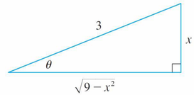
Since this is an indefinite integral, we must return to the original variable x. This can be done either by using trigonometric identities to express $\cot\theta$ in terms of $\sin\theta = x/3$ or by drawing a diagram, as in Figure 8.3, where $\theta$ is interpreted as an angle of a right triangle.

Figure 8.3: sin θ = x/3

Based on the Pythagorean Theorem, the length of the adjacent side can be expressed as

$\sqrt{9-x^2}$

Then, we can simply read the value of $\cot\theta$ from the figure:

$\cot\theta = \frac{\sqrt{9-x^2}}{x}$

(Although $\theta > 0$ in the diagram, this expression for $\cot\theta$ is valid even when $\theta < 0$). Since $\sin\theta = x/3$, then $\theta = \sin^{-1}(x/3)$. Therefore

$\int \frac{\sqrt{9-x^2}}{x^2}\,dx = -\frac{\sqrt{9-x^2}}{x} - \sin^{-1}\left(\frac{x}{3}\right) + C$

Example 8.6

Find

$\int \frac{x^3}{\sqrt{9-x^2}}\,dx$

Solution

Lets, x = 3 sin t

$$\begin{aligned} &= 27\int \frac{\sin^3 t \cos t}{\sqrt{1-\sin^2 t}}\,dt \\ &= 27\int \sin^3 t\,dt \\ &= 27\int (1-\cos^2 t)\sin t\,dt \\ &= 27\left(-\cos t + \frac{\cos^3 t}{3}\right) + C \\ &= 27\left(-\sqrt{1-\sin^2 t} + \frac{1}{3}(1-\sin^2 t)^{3/2}\right) + C \\ &= -9\sqrt{9-x^2} + \frac{1}{3}(9-x^2)^{3/2} + C \end{aligned}$$

Where, x = 3 sin t , dx = 3 cos t dt

8.2.3 Partial Fractions

This section demonstrates a method to integrate any rational function (a ratio of polynomials) by expressing it as a sum of simpler fractions, called partial fractions, that we already know how to integrate.

To illustrate the method, observe that by taking the fractions $\dfrac{2}{(x-1)}$ and $\dfrac{1}{(x+2)}$ to a common denominator, the expression becomes

$$\begin{aligned} \frac{2}{(x-1)} - \frac{1}{(x+2)} &= \frac{2(x+2) - (x-1)}{(x-1)(x+2)} \\ &= \frac{x+5}{x^2+x-2} \end{aligned}$$

If we reverse the procedure, we see how to integrate the function on the right side of the following equation.

$$\begin{aligned} \int \frac{x+5}{x^2+x-2}\,dx &= \int \left(\frac{2}{(x-1)} - \frac{1}{(x+2)}\right)dx \\ &= 2\ln\lvert x-1\rvert - \ln\lvert x+2\rvert + C \end{aligned}$$

In order to illustrate the method, let

$f(x) = \frac{P(x)}{Q(x)}$

Be a rational function where $P(x)$ and $Q(x)$ are polynomials. The function $f(x)$ can be expressed as a sum of simpler fractions provided that the degree of P is less than the degree of Q. Such a rational function is called proper.

If,

$P(x) = a_n x^n + a_{n-1}x^{n-1} + \cdots + a_1 x + a_0$

Where $a_n \neq 0$, then the degree of P is n and we write deg(P) = n. If f is improper, that is, deg(P) $\geq$ deg(Q), then we must take the preliminary step of dividing Q into P (by long division) until a remainder R (x) is obtained such that deg(R) < deg(Q).

The division statement is

$f(x) = \frac{P(x)}{Q(x)} = S(x) + \frac{R(x)}{Q(x)} \qquad \ldots\ldots(4)$

where S and R are also polynomials.

As the next example illustrates, sometimes this preliminary step is all that is required.

Example 8.7

Find

$\int \frac{x^3+x}{x-1}\,dx$

Solution

Since the degree of the numerator is greater than the degree of the denominator, we first perform the long division.

$$\begin{aligned} \int \frac{x^3+x}{x-1}\,dx &= \int \left(x^2 + x + 2 + \frac{2}{x-1}\right)dx \\ &= \frac{x^3}{3} + \frac{x^2}{2} + 2x + 2\ln\lvert x-1\rvert + C \end{aligned}$$

From Eq (4), if the denominator is more complicated, then the next step is to factor the denominator Q (x) as far as possible. It can be shown that any polynomial Q can be factored as a product of linear factors (of the form $ax + b$) and irreducible quadratic factors (of the form $ax^2+bx+c$, where $b^2-4ac<0$).

For example, if $Q(x) = x^4-16$, we could factor it as

$Q(x) = (x^2-4)(x^2+4) = (x-2)(x+2)(x^2+4)$

Then, the next step is to express the proper rational function $R(x)/Q(x)$ in Eq (4) as a sum of partial fractions of the following form

$\frac{A}{(ax+b)^i} \qquad \text{or} \qquad \frac{Ax+B}{(ax^2+bx+c)^j}$

A theorem in algebra guarantees that it is always possible to do this. We explain the details for the four cases that occur:

a) The denominator $Q(x)$ is a product of distinct linear factors

b) $Q(x)$ is a product of linear factors, some of which are repeated

c) $Q(x)$ contains irreducible quadratic factors, none of which is repeated

d) $Q(x)$ contains a repeated irreducible quadratic factor

8.2.3.1 Case 1: Q(x) is a Product of Distinct Linear Factors

For this case, we could expressed $Q(x)$ as

$Q(x) = (a_1x+b_1)(a_2x+b_2) \ldots (a_kx+b_k),$

Where no factor is repeated and no factor is a constant multiple of another. Hence, in this case, the partial fraction theorem states that there exist constant $A_1, A_2, \ldots, A_k$ such that

$\frac{R(x)}{Q(x)} = \frac{A_1}{a_1x+b_1} + \frac{A_2}{a_2x+b_2} + \cdots + \frac{A_k}{a_kx+b_k} \qquad \ldots\ldots(5)$

Example 8.8

Evaluate

$\int \frac{x^2+2x-1}{2x^3+3x^2-2x}\,dx$

Solution

Since the degree of the numerator is less than the degree of the denominator, we don't need to divide. We factor the denominator as

$$\begin{aligned} 2x^3+3x^2-2x &= x(2x^2+3x-2) \\ &= x(2x-1)(x+2) \end{aligned}$$

Then,

$\frac{x^2+2x-1}{x(2x-1)(x+2)} = \frac{A}{x} + \frac{B}{2x-1} + \frac{C}{x+2}$

In order to determine the constant $A$, $B$ and C, multiply both sides of the equation by the product of the denominators to give

$$\begin{aligned} x^2+2x-1 &= A(2x-1)(x+2) + Bx(x+2) + Cx(2x-1) \\ &= (2A+B+2C)x^2 + (3A+2B-C)x - 2A \end{aligned}$$

System of equations:

$2A + B + 2C = 1$

$3A + 2B - C = 2$

$-2A = -1$

Thus, $A = \dfrac{1}{2}$, $B = \dfrac{1}{5}$, $C = -\dfrac{1}{10}$

$$\begin{aligned} \int \frac{x^2+2x-1}{2x^3+3x^2-2x}\,dx &= \int \left(\frac{1}{2}\frac{1}{x} + \frac{1}{5}\frac{1}{2x-1} - \frac{1}{10}\frac{1}{x+2}\right)dx \\ &= \frac{1}{2}\ln\lvert x\rvert + \frac{1}{10}\ln\lvert 2x-1\rvert - \frac{1}{10}\ln\lvert x+2\rvert + K \end{aligned}$$

Note that in integrating the middle term, the following substitutions have been made:

$u = 2x-1, \qquad du = 2dx, \qquad \text{then } dx = \frac{1}{2}du$

8.2.3.2 Case 2: Q(x) is a Product of Distinct Linear Factors, Some of Which Are Repeated

Suppose the first linear factor $(a_1x+b_1)$ is repeated $r$ times, that is, $(a_1x+b_1)^r$ occurs in the factorization of $Q(x)$. Then, instead of the single term in Eq (5), we could use

$\frac{A_1}{a_1x+b_1} + \frac{A_2}{(a_1x+b_1)^2} + \cdots + \frac{A_r}{(a_1x+b_1)^r} \qquad \ldots\ldots(6)$

Example 8.9

Find

$\int \frac{x^4-2x^2+4x+1}{x^3-x^2-x+1}\,dx$

Solution

The first step is to divide using long division, which gives

$\frac{x^4-2x^2+4x+1}{x^3-x^2-x+1} = x + 1 + \frac{4x}{x^3-x^2-x+1}$

The next step is to factor out the denominator

$$\begin{aligned} x^3-x^2-x+1 &= (x-1)(x^2-1) \\ &= (x-1)(x-1)(x+1) \\ &= (x-1)^2(x+1) \end{aligned}$$

Hence,

$\frac{4x}{(x-1)^2(x+1)} = \frac{A}{x-1} + \frac{B}{(x-1)^2} + \frac{C}{x+1}$

$4x = A(x-1)(x+1) + B(x+1) + C(x-1)^2$

Equate coefficients, we obtain $A = 1$, $B = 2$, $C = -1$. Hence,

$$\begin{aligned} \int \frac{x^4-2x^2+4x+1}{x^3-x^2-x+1}\,dx &= \int \left[x + 1 + \frac{1}{x-1} + \frac{2}{(x-1)^2} - \frac{1}{x+1}\right]dx \\ &= \frac{x^2}{2} + x + \ln\lvert x-1\rvert - \frac{2}{x-1} - \ln\lvert x+1\rvert + K \\ &= \frac{x^2}{2} + x - \frac{2}{x-1} + \ln\left\lvert\frac{x-1}{x+1}\right\rvert + K \end{aligned}$$

Try this

Please integrate, $\displaystyle \int \frac{x^2 - x + 1}{(x+1)^3}\,dx$

Solution

$\ln\lvert x+1\rvert + \frac{3}{x+1} - \frac{3}{2(x+1)^2} + C.$

8.2.3.3 Case 3: Q(x) Contains Irreducible Quadratic Factors, None of Which is Repeated

If $Q(x)$ has the factor $ax^2+bx+c$, where $b^2-4ac<0$, then, in addition to the partial fractions in Eq (5) and (6), the expression for $R(x)/Q(x)$ will have a term of the form

$\frac{Ax+B}{ax^2+bx+c} \qquad \ldots\ldots(7)$

Where A and B are constants to be determined. The term in Eq (7) can be integrated by completing squares (if necessary) and using the following formula

$\int \frac{dx}{x^2+a^2} = \frac{1}{a}\tan^{-1}\left(\frac{x}{a}\right) + C$

Example 8.10

Evaluate

$\int \frac{4x^2-3x+2}{4x^2-4x+3}\,dx$

Solution

Since the degree of the numerator is not less than the degree of the denominator, we divide the expression, which yield

$\frac{4x^2-3x+2}{4x^2-4x+3} = 1 + \frac{x-1}{4x^2-4x+3}$

Note that the quadratic $4x^2-4x+3$ is irreducible because its discriminant $b^2-4ac = -32 < 0$. Hence, we complete the square

$4x^2-4x+3 = (2x-1)^2 + 2$

Let

$u = 2x-1, \quad du = 2dx, \quad x = \frac{1}{2}(u+1)$

Hence,

$$\begin{aligned} \int \frac{4x^2-3x+2}{4x^2-4x+3}\,dx &= \int \left(1 + \frac{x-1}{4x^2-4x+3}\right)dx \\ &= x + \frac{1}{2}\int \frac{\frac{1}{2}(u+1) - 1}{u^2+2}\,du \\ &= x + \frac{1}{4}\int \frac{u-1}{u^2+2}\,du \\ &= x + \frac{1}{4}\int \frac{u}{u^2+2}\,du - \frac{1}{4}\int \frac{1}{u^2+2}\,du \\ &= x + \frac{1}{8}\ln(u^2+2) - \frac{1}{4}\cdot\frac{1}{\sqrt{2}}\tan^{-1}\left(\frac{u}{\sqrt{2}}\right) + C \\ &= x + \frac{1}{8}\ln(4x^2-4x+3) - \frac{1}{4\sqrt{2}}\tan^{-1}\left(\frac{2x-1}{\sqrt{2}}\right) + C \end{aligned}$$

Try this

Please integrate $\displaystyle \int \frac{3x+1}{x^2(x^2+25)}\,dx$

Solution

$\frac{3}{25}\ln\lvert x\rvert - \frac{1}{25x} - \frac{3}{50}\ln\lvert x^2+25\rvert - \frac{1}{125}\arctan\frac{x}{5} + C$

8.2.3.4 Case 4: Q(x) Contains a Repeated Irreducible Quadratic Factor

If $Q(x)$ has the factor $(ax^2+bx+c)^r$, where $b^2-4ac<0$, then

$\frac{A_1x+B_1}{ax^2+bx+c} + \frac{A_2x+B_2}{(ax^2+bx+c)^2} + \cdots + \frac{A_rx+B_r}{(ax^2+bx+c)^r} \qquad \ldots\ldots(8)$

occurs in the partial fraction decomposition of $R(x)/Q(x)$. Each of the terms in Eq (8) can be integrated using a substitution or by first completing the square if necessary.

Example 8.11

Evaluate

$\int \frac{1-x+2x^2-x^3}{x(x^2+1)^2}\,dx$

Solution

The form of the partial fraction decomposition is

$\frac{1-x+2x^2-x^3}{x(x^2+1)^2} = \frac{A}{x} + \frac{Bx+C}{x^2+1} + \frac{Dx+E}{(x^2+1)^2}$

Then

$$\begin{aligned} -x^3+2x^2-x+1 &= A(x^2+1)^2 + (Bx+C)x(x^2+1) + (Dx+E)x \\ &= (A+B)x^4 + Cx^3 + (2A+B+D)x^2 + (C+E)x + A \end{aligned}$$

Equating coefficients, we obtain $A = 1$, $B = -1$, $C = -1$, $D = 1$, $E = 0$.

$$\begin{aligned} \int \frac{1-x+2x^2-x^3}{x(x^2+1)^2}\,dx &= \int \left(\frac{1}{x} - \frac{x+1}{x^2+1} + \frac{x}{(x^2+1)^2}\right)dx \\ &= \int \frac{dx}{x} - \int \frac{x}{x^2+1}dx - \int \frac{dx}{x^2+1} + \int \frac{x\,dx}{(x^2+1)^2} \\ &= \ln\lvert x\rvert - \frac{1}{2}\ln(x^2+1) - \tan^{-1}x - \frac{1}{2(x^2+1)} + K \end{aligned}$$

---

8.3 Improper Integrals

In this sub section, extend the concept of a definite integral to the case where the interval is infinite and also to the case where f has an infinite discontinuity in [a, b]. In either case the integral is called an improper integral

8.3.1 Type 1: Infinite Intervals

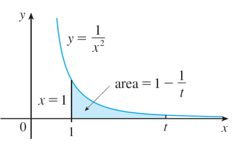
Consider the infinite region $\mathcal{S}$ that lies under the curve $y = 1/x^2$, above the x-axis, and to the right of line $x = 1$. This is shown in Figure 8.4.

Figure 8.4: y = 1/x²

You might think that since $\mathcal{S}$ is infinite in extent, its area must be infinite, but let's take a closer look. From Figure 8.4, we can see that the area of the part of $\mathcal{S}$ that lies to the left of the line $x = t$ (shaded area) is

$$\begin{aligned} A(t) &= \int_1^t \frac{1}{x^2}\,dx = -\frac{1}{x}\Big]_1^t \\ &= 1 - \frac{1}{t} \end{aligned}$$

Notice that $A(t) < 1$ no matter how large $t$ is chosen. We also observe that

$\lim_{t\to\infty} A(t) = \lim_{t\to\infty}\left(1 - \frac{1}{t}\right) = 1$

This is shown in Figure 8.5.

Figure 8.5: Area under the curve as t → ∞

Using this example as a guide, we define the integral of f over an infinite interval as the limit of integrals over finite intervals. The definition of an improper integral of Type 1 is given below.

Definition of an Improper Integral of Type 1

(a) If $\displaystyle \int_a^t f(x)\,dx$ exists for every number $t \geq a$, then

$\int_a^{\infty} f(x)\,dx = \lim_{t\to\infty}\int_a^t f(x)\,dx$

provided this limit exists (as a finite number).

(b) If $\displaystyle \int_t^b f(x)\,dx$ exists for every number $t \leq b$, then

$\int_{-\infty}^{b} f(x)\,dx = \lim_{t\to-\infty}\int_t^b f(x)\,dx$

provided this limit exists (as a finite number).

The improper integrals $\displaystyle \int_a^{\infty} f(x)\,dx$ and $\displaystyle \int_{-\infty}^{b} f(x)\,dx$ are called convergent if the corresponding limit exists and divergent if the limit does not exist.

(c) If both $\displaystyle \int_a^{\infty} f(x)\,dx$ and $\displaystyle \int_{-\infty}^{a} f(x)\,dx$ are convergent, then we define

$\int_{-\infty}^{\infty} f(x)\,dx = \int_{-\infty}^{a} f(x)\,dx + \int_a^{\infty} f(x)\,dx$

In part (c) any real number $a$ can be used

Example 8.12

Determine whether the integral $\displaystyle \int_1^{\infty}\left(\frac{1}{x}\right)dx$ is convergent or divergent

Solution

$$\begin{aligned} \int_1^{\infty}\left(\frac{1}{x}\right)dx &= \lim_{t\to\infty}\ln\lvert x\rvert\Big]_1^t = \lim_{t\to\infty}(\ln t - \ln 1) \\ &= \lim_{t\to\infty}\ln t = \infty \end{aligned}$$

The limit does not exist as a finite number and so the improper integral is divergent.

8.3.2 Type 2: Discontinuous Integrands

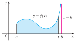
Suppose that $f$ is a positive continuous function defined on a finite interval [a, b) but has a vertical asymptote at b. Let S be the unbounded region under the graph of f and above the x-axis between a and b. (For Type 1 integrals, the regions extended indefinitely in a horizontal direction. Here the region is infinite in a vertical direction.)

The area of the part of S between a and t (the shaded region in Figure 8.7) is

$A(t) = \int_a^t f(x)dx$

Figure 8.7: Area of the part of S

If it happen that $A(t)$ approaches a definite number $A$ as $t \to b^-$, then we say that the area of the region S is $A$ and we could write

$\int_a^b f(x)dx = \lim_{t\to b^-}\int_a^t f(x)dx$

We use this equation to define an improper integral of Type 2 even when $f$ is not a positive function, no matter what type of discontinuity $f$ has at b. The definition of an improper integral of Type 2 is given below.

Definition of an Improper Integral of Type 2

(a) If $f$ is continuous on $[a, b)$ and is discontinuous at $b$, then

$\int_a^b f(x)\,dx = \lim_{t\to b^-}\int_a^t f(x)\,dx$

if this limit exists (as a finite number).

(b) If $f$ is continuous on $(a, b]$ and is discontinuous at $a$, then

$\int_a^b f(x)\,dx = \lim_{t\to a^+}\int_t^b f(x)\,dx$

if this limit exists (as a finite number).

The improper integral $\displaystyle \int_a^b f(x)\,dx$ is called convergent if the corresponding limit exists and divergent if the limit does not exist.

(c) If $f$ has a discontinuity at $c$, where $a < c < b$, and both $\displaystyle \int_a^c f(x)\,dx$ and $\displaystyle \int_c^b f(x)\,dx$ are convergent, then we define

$\int_a^b f(x)\,dx = \int_a^c f(x)\,dx + \int_c^b f(x)\,dx$

Example 8.13

Find

$\int_2^5 \frac{1}{\sqrt{x-2}}\,dx$

Solution

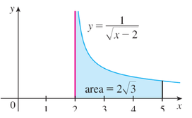
The given integral is improper because $f(x) = \dfrac{1}{\sqrt{x-2}}$ has the vertical asymptote at $x = 2$. Since the infinite discontinuity occurs at the left endpoint of [2, 5], we use part (b) of the definition of an improper integral of Type 2.

$$\begin{aligned} \int_2^5 \frac{1}{\sqrt{x-2}}\,dx &= \lim_{t\to 2^+}\int_t^5 \frac{dx}{\sqrt{x-2}} \\ &= \lim_{t\to 2^+} 2\sqrt{x-2}\Big]_t^5 = \lim_{t\to 2^+}\left(2\sqrt{3} - 2\sqrt{t-2}\right) \\ &= 2\sqrt{3} \end{aligned}$$

Thus the given improper integral is convergent and, since the integrand is positive, we can interpret the value of the integral as the area of the shaded region in Figure 8.9.

Figure 8.9: y = 1/√(x-2)

8.3.3 A Comparison Test for Improper Integrals

Sometimes it is impossible to find the exact value of an improper integral and yet it is important to know whether it is convergent or divergent.

In such cases the following theorem is useful. Although we state it for Type 1 integrals, a similar theorem is true for Type 2 integrals.

Comparison Theorem

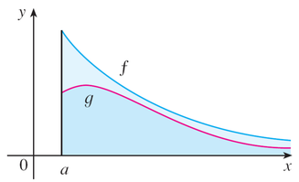
Suppose that $f$ and $g$ are continuous functions with $f(x) \geq g(x) \geq 0$ for $x \geq a$.

(a) If $\displaystyle \int_a^{\infty} f(x)\,dx$ is convergent, then $\displaystyle \int_a^{\infty} g(x)\,dx$ is convergent.

(b) If $\displaystyle \int_a^{\infty} g(x)\,dx$ is divergent, then $\displaystyle \int_a^{\infty} f(x)\,dx$ is divergent.

We omit the proof of the Comparison Theorem, but Figure 8.10 makes it seem plausible.

Figure 8.10: Area under the curve

If the area under the top curve y = f (x) is finite, then so is the area under the bottom curve y = g (x).

If the area under y = g (x) is infinite, then so is the area under y = f (x). [Note that the reverse is not necessarily true: If $\displaystyle \int_a^{\infty} g(x)dx$ is convergent, $\displaystyle \int_a^{\infty} f(x)dx$ may or may not be convergent, and if $\displaystyle \int_a^{\infty} f(x)dx$ is divergent, $\displaystyle \int_a^{\infty} g(x)dx$ may or may not be divergent.]