Lecture 9: Engineering Application of Integrals

Download the original PDF →


9.1 (I) Area Between Curves​

In this section we will determine the area of a region between two curves by integrating with respect to the independent variable. The area of a region between two curves will also be determined using definite integration with respect to the dependent variable. We also try to find the area of a compound region.

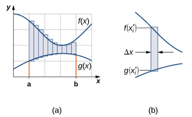
Let f(x)f(x) and g(x)g(x) be continuous functions over an interval [a,b][a,b] such that f(x)≥g(x)f(x) \ge g(x) on [a,b][a,b]. We want to find the area between the graphs of the functions, as shown in Figure 9.1.

Figure 9.1: The area between the graphs of two functions, f(x) and g(x), on the interval [a,b]

Figure 9.1: The area between the graphs of two functions, f(x) and g(x), on the interval [a,b]

As we did before, we are going to partition the interval on the xx-axis and approximate the area between the graphs of the functions with rectangles. So, for i=0,1,2,…,ni=0,1,2,\dots,n, let P=xiP=x_i be a regular partition of [a,b][a,b]. Then, for i=1,2,…,ni=1,2,\dots,n, choose a point xi∗∈[xi−1,xi]x_i^* \in [x_{i-1},x_i], and on each interval [xi−1,xi][x_{i-1},x_i] construct a rectangle that extends vertically from g(xi∗)g(x_i^*) to f(xi∗)f(x_i^*). Figure 9.2(a) shows the rectangles when xi∗x_i^* is selected to be the left endpoint of the interval and n=10n=10. Figure 9.2(b) shows a representative rectangle in detail.

Figure 9.2: (a) We can approximate the area between the graphs of two functions, f(x) and g(x), with rectangles. (b) The area of a typical rectangle goes from one curve to the other.

Figure 9.2: (a) We can approximate the area between the graphs of two functions, f(x) and g(x), with rectangles. (b) The area of a typical rectangle goes from one curve to the other.

The height of each individual rectangle is f(xi∗)−g(xi∗)f(x_i^*)-g(x_i^*) and the width of each rectangle is Δx\Delta x. Adding the areas of all the rectangles, we see that the area between the curves is approximated by:

A≈∑i=1n[f(xi∗)−g(xi∗)]Δx(9.1)A \approx \sum_{i=1}^{n}[f(x_i^*)-g(x_i^*)]\Delta x \qquad (9.1)

This is a Riemann sum, so we take the limit as n→∞n \to \infty and we get,

A=lim⁡n→∞∑i=1n[f(xi∗)−g(xi∗)]Δx=∫ab[f(x)−g(x)] dx(9.2)A = \lim_{n \to \infty}\sum_{i=1}^{n}[f(x_i^*)-g(x_i^*)]\Delta x = \int_a^b[f(x)-g(x)]\,dx \qquad (9.2)

In conclusion, let f(x)f(x) and g(x)g(x) be continuous functions such that f(x)≥g(x)f(x) \ge g(x) over an interval [a,b][a,b]. Let "RR" denote the region bounded above by the graph of f(x)f(x), below by the graph of g(x)g(x), and on the left and right by the lines x=ax=a and x=bx=b, respectively. Then, the area of "RR" is given by,

A=∫ab[f(x)−g(x)] dx(9.3)A = \int_a^b[f(x)-g(x)]\,dx \qquad (9.3)

Example 9.1​

Find the area bounded by two curves, f(x)=−x2+4x+3f(x) = -x^2+4x+3 and g(x)=−x3+7x2−10x+5g(x) = -x^3+7x^2-10x+5 over the interval 1≤x≤21 \le x \le 2.

Solution

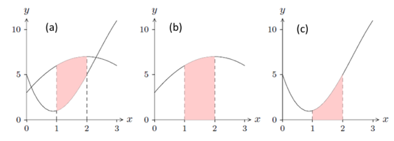
The region can be depicted as shown in Figure 9.3(a) with the desired area shaded. Also, we can depict ff alone with the area under ff shaded, and then gg alone with the area under gg shaded.

Figure 9.3: Area between curves as a difference of areas

Figure 9.3: Area between curves as a difference of areas

It is clear from the figure that the area we want is the area under ff minus the area under gg, which can be written as,

A=∫12f(x) dx−∫12g(x) dx=∫12[f(x)−g(x)] dx=∫12[(−x2+4x+3)−(−x3+7x2−10x+5)]dx=x44−8x33+7x2−2x∣12=4912\begin{aligned} A &= \int_1^2 f(x)\,dx - \int_1^2 g(x)\,dx = \int_1^2[f(x)-g(x)]\,dx \\ &= \int_1^2\left[(-x^2+4x+3)-(-x^3+7x^2-10x+5)\right]dx \\ &= \frac{x^4}{4} - \frac{8x^3}{3} + 7x^2 - 2x \Big|_1^2 \\ &= \frac{49}{12} \end{aligned}

Example 9.2​

If RR is the region bounded above by the graph of the function f(x)=9−(x/2)2f(x) = 9-(x/2)^2 and below by the graph of the function g(x)=6−xg(x) = 6-x, find the area of region RR.

Solution

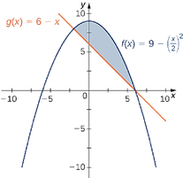
The region can be depicted by the following figure.

Figure 9.4: This graph shows the region below the graph of f(x) and above the graph of g(x)

Figure 9.4: This graph shows the region below the graph of f(x) and above the graph of g(x).

We first need to compute where the graphs of the functions intersect. Setting f(x)=g(x)f(x)=g(x), we get,

f(x)=g(x)9−(x2)2=6−x36−x2=24−4x(x−6)(x+2)=0x=(6,−2)\begin{aligned} f(x) &= g(x) \\ 9 - \left(\frac{x}{2}\right)^2 &= 6-x \\ 36 - x^2 &= 24 - 4x \\ (x-6)(x+2) &= 0 \\ x &= (6,-2) \end{aligned}

The graphs of the functions intersect when x=6x=6 or x=−2x=-2, so we want to integrate from −2-2 to 66. Since f(x)≥g(x)f(x) \ge g(x) for −2≤x≤6-2 \le x \le 6, we obtain,

A=∫ab[f(x)−g(x)] dx=∫−26[9−(x2)2−(6−x)]dx=∫−26[3−x24+x]dx=[3x−x312+x22]−26=643\begin{aligned} A &= \int_a^b[f(x)-g(x)]\,dx \\ &= \int_{-2}^{6}\left[9-\left(\frac{x}{2}\right)^2-(6-x)\right]dx \\ &= \int_{-2}^{6}\left[3-\frac{x^2}{4}+x\right]dx \\ &= \left[3x-\frac{x^3}{12}+\frac{x^2}{2}\right]_{-2}^{6} = \frac{64}{3} \end{aligned}

9.1 (II) Areas of Compound Regions​

So far, we have required, f(x)≥g(x)f(x) \ge g(x) over the entire interval of interest, but what if we want to look at regions bounded by the graphs of functions that cross one another? In that case, we modify the process we just developed by using the absolute value function.

Example 9.3: Finding the Area of a Region Bounded by Functions That Cross​

If RR is the region between the graphs of the functions f(x)=sin⁡xf(x) = \sin x and g(x)=cos⁡xg(x) = \cos x over the interval [0,π][0,\pi], find the area of region RR.

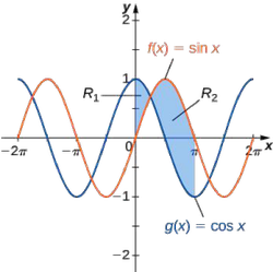
The region can be depicted by the following figure.

Figure 9.5: The region between two curves can be broken into two sub-regions

Figure 9.5: The region between two curves can be broken into two sub-regions.
Solution

The graphs of the functions intersect at x=π/4x = \pi/4. For x∈[0,π/4]x \in [0,\pi/4], cos⁡x≥sin⁡x\cos x \ge \sin x, thus,

∣f(x)−g(x)∣=∣sin⁡x−cos⁡x∣=cos⁡x−sin⁡x|f(x)-g(x)| = |\sin x - \cos x| = \cos x - \sin x

On the other hand, for x∈[π/4,π]x \in [\pi/4,\pi], sin⁡x≥cos⁡x\sin x \ge \cos x, thus,

∣f(x)−g(x)∣=∣sin⁡x−cos⁡x∣=sin⁡x−cos⁡x|f(x)-g(x)| = |\sin x - \cos x| = \sin x - \cos x

Now,

A=∫ab[f(x)−g(x)] dx=∫0π∣sin⁡x−cos⁡x∣ dx=∫0π/4[cos⁡x−sin⁡x] dx+∫π/4π[sin⁡x−cos⁡x] dx=(2−1)+(1+2)=22\begin{aligned} A &= \int_a^b[f(x)-g(x)]\,dx \\ &= \int_0^{\pi}|\sin x - \cos x|\,dx \\ &= \int_0^{\pi/4}[\cos x - \sin x]\,dx + \int_{\pi/4}^{\pi}[\sin x - \cos x]\,dx \\ &= (\sqrt{2}-1) + (1+\sqrt{2}) \\ &= 2\sqrt{2} \end{aligned}

Example 9.4​

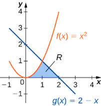
Consider the region depicted in Figure 9.6. Find the area of RR.

Figure 9.6: Two integrals are required to calculate the area of this region

Figure 9.6: Two integrals are required to calculate the area of this region.
Solution

As with Example 9.3, we need to divide the interval into two pieces. The graphs of the functions intersect at x=1x=1 (set f(x)=g(x)f(x)=g(x) and solve for xx), so we evaluate two separate integrals: one over the interval [0,1][0,1] and one over the interval [1,2][1,2].

Over the interval [0,1][0,1], the region is bounded above by f(x)=x2f(x)=x^2 and below by the xx-axis, so we have,

A1=∫01x2 dx=x33=13A1 = \int_0^1 x^2\,dx = \frac{x^3}{3} = \frac{1}{3}

Over the interval [1,2][1,2], the region is bounded above by g(x)=2−xg(x)=2-x and below by the xx-axis, so we have,

A2=∫12(2−x) dx=12A2 = \int_1^2(2-x)\,dx = \frac{1}{2}

Adding these areas together, we obtain, A=A1+A2=5/6A = A1+A2 = 5/6

The area of the region is, 5/65/6 units².

9.2 Hydrostatic Force​

In this section, we will learn about the force exerted by a fluid on a horizontal surface. Also, we will determine the hydrostatic force against a vertical surface.

9.2 (I) Force Exerted by a Fluid on a Horizontal Surface​

Deep-sea divers know that pressure increases as they swim deeper because their bodies have to support larger volumes of water. If a planar plate with an area of AA square meters is submerged horizontally in a fluid at a depth of dd meters, as in Figure 9.7, then the volume of the fluid above the plate is V=AdV = Ad. Moreover, the mass mm of the fluid above the plate is m=Vωm = V\omega where ω\omega is the mass density of the fluid in kilograms per cubic meter. Applying Newton's Second Law of Motion, the force exerted by the fluid on the plate is:

Force=mg=Adωg\text{Force} = mg = Ad\omega g

Figure 9.7: A plate of area A is submerged horizontally in a fluid of depth d

Figure 9.7: A plate of area A is submerged horizontally in a fluid of depth d.

Where, gg is the acceleration due to gravity. The product ω′=ωg\omega' = \omega g is called the weight density of the fluid, and is the weight per unit volume of the fluid. Then the force exerted by the fluid on the plate at a depth dd meters is given by:

Force=(Area)⋅(Depth)⋅(Weight Density)=Adω′\text{Force} = (\text{Area}) \cdot (\text{Depth}) \cdot (\text{Weight Density}) = Ad\omega'

Consequently, the pressure or force per unit area weighing on the horizontal plate is defined as:

Pressure=ForceArea=dω′\text{Pressure} = \frac{\text{Force}}{\text{Area}} = d\omega'

The above equation implies that the pressure is directly proportional to the depth. This is why a deep-sea diver experiences more pressure as he or she swims deeper.

9.2 (II) Hydrostatic Force Against a Vertical Surface​

Early in the section, we described the force exerted by a fluid on a horizontal surface without using calculus, see §9.2 (I). However, in order to find the force exerted by a fluid on a vertical surface we have to apply calculus. In addition, we apply a physical principle due to Blaise Pascal, i.e., at a fixed depth a fluid exerts the same pressure in all directions.

We draw a yy-axis so that the depths of a vertical surface vary from points y=cy = c to y=dy = d on the yy-axis. Then partition [c,d][c,d] into nn subintervals of equal width Δy\Delta y. If Δy\Delta y is small, the portion of the vertical plate associated to the iith subinterval [yi−1,yi][y_{i-1},y_i] is approximately a vertical rectangular strip RiR_i of length L(yi)L(y_i) and width Δy\Delta y. Moreover, the depth of RiR_i from the surface of the fluid is almost constant and which we denote by d(yi)d(y_i). Applying the above principle due to Pascal, the force FiF_i exerted by the fluid on a vertical rectangle RiR_i is approximately:

Fi≈Area . Depth . Weight densityF_i \approx Area\,.\,Depth\,.\,Weight\ density

≈[L(yi)Δy] d(yi) ω′\approx [L(y_i)\Delta y]\,d(y_i)\,\omega'

We find it reasonable to believe that the sum of the FiF_i's approximates the force FF exerted by the fluid on the entire vertical surface, i.e.,

F≈∑i=1nFi=∑i=1n[L(yi)Δy] d(yi) ω′F \approx \sum_{i=1}^{n}F_i = \sum_{i=1}^{n}[L(y_i)\Delta y]\,d(y_i)\,\omega'

Suppose a yy-axis is positioned vertically so that the depths of the fluid vary from points y=cy = c to y=dy = d on the yy-axis. At point yy in [c,d][c,d], let d(y)d(y) and L(y)L(y) be the depth and length from side to side of the surface, respectively. The force exerted by the fluid on one side of the vertical surface is given by:

F=∫cdL(y) . d(y) . dy(9.4)F = \int_c^d L(y)\,.\,d(y)\,.\,dy \qquad (9.4)

provided d(y)d(y) and L(y)L(y) are continuous functions of yy.

Example 9.5​

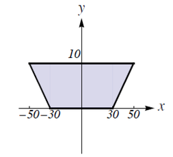
A vertical dam has a cross section that is a trapezoid, see Figure 9.8. The dimensions of the trapezoid are 10 meters high, 100 meters across the top, and the base is 60 meters. If the dam is filled with water, find the force exerted by the water on the cross section.

Solution

Figure 9.8: The cross section of a vertical dam

Figure 9.8: The cross section of a vertical dam.

Since water has a mass density of 1000 kg/m31000\ \text{kg/m}^3 and gravity is 9.8 m/sec29.8\ \text{m/sec}^2, the weight density of water is:

ω′=1000⋅9.8=9800 kgm2sec2\omega' = 1000 \cdot 9.8 = 9800\ \frac{kg}{m^2sec^2}

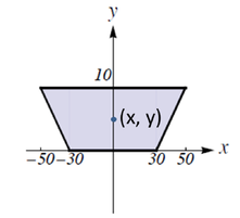
Figure 9.9: The cross section of a vertical dam

Figure 9.9: The cross section of a vertical dam

Let consider (x,y)(x,y) is the center of the base of the dam. An equation of the slanted side of the dam in the first quadrant is:

y=x2−15y = \frac{x}{2} - 15

x=2y+30x = 2y + 30

At point yy in [0,10][0,10], the horizontal distance across the dam is:

L(y)=2x=4y+60L(y) = 2x = 4y + 60

and the water depth is: d(y)=10−yd(y) = 10-y

Now,

Force=ω′∫cdL(y)d(y) dy=9800∫010(4y+60)(10−y) dyForce = \omega'\int_c^d L(y)d(y)\,dy = 9800\int_0^{10}(4y+60)(10-y)\,dy

=3.593×10⁷ kg . msec2= 3.593 \times 10^7\ \frac{kg\,.\,m}{sec^2}

Example 9.6​

A dam has the shape of the trapezoid shown in Figure 9.10. The height is 20 m and the width is 50 m at the top and 30 m at the bottom. Find the force on the dam due to hydrostatic pressure if the water level is 4 m from the top of the dam.

Figure 9.10: A dam with shape of trapezoid

Figure 9.10: A dam with shape of trapezoid
Solution
  • Choose a vertical xx-axis with origin at the surface of the water and directed downward
  • Divide the depth of water into intervals between [0,16][0,16] of equal length
  • At the iith strip (x=xi∗)(x = x_i^*),

a16−xi∗=1020\frac{a}{16-x_i^*} = \frac{10}{20}

From which,

a=16−xi∗2=8−xi∗2a = \frac{16-x_i^*}{2} = 8 - \frac{x_i^*}{2}

Width of the dam at the iith strip, wiw_i can be found by,

wi=2(15+a)=2(15+8−xi∗2)=46−xi∗w_i = 2(15+a) = 2\left(15+8-\frac{x_i^*}{2}\right) = 46-x_i^*

  • At the iith strip, the area AiA_i can be approximated by,

Ai≈wiΔx=(46−xi∗)ΔxA_i \approx w_i\Delta x = (46-x_i^*)\Delta x

  • When Δx\Delta x is small, the pressure acting on the iith strip, PiP_i is almost constant:

Pi≈1000gxi∗P_i \approx 1000gx_i^*

  • The hydrostatic force on the iith strip, FiF_i,

Fi=PiAi≈1000gxi∗(46−xi∗)ΔxF_i = P_iA_i \approx 1000gx_i^*(46-x_i^*)\Delta x

  • Adding these forces and taking the limit as n→∞n \to \infty,
F=lim⁡n→∞∑i=1n1000gxi∗(46−xi∗)Δx=∫0161000gx(46−x) dx=1000(9.8)∫016(46x−x2) dx=9800[23x2−x33]016≈4.43×10⁷ N\begin{aligned} F &= \lim_{n \to \infty}\sum_{i=1}^{n}1000gx_i^*(46-x_i^*)\Delta x \\ &= \int_0^{16}1000gx(46-x)\,dx \\ &= 1000(9.8)\int_0^{16}(46x-x^2)\,dx \\ &= 9800\left[23x^2-\frac{x^3}{3}\right]_0^{16} \\ &\approx 4.43 \times 10^7\ N \end{aligned}

Example 9.7​

A circular plate with a radius of 1 ft is submerged vertically in a tank filled with water. The center of the plate is 4 ft from the surface of the water. Find the force exerted by the water on one side of the plate.

Figure 9.11: A plate with a circular cross section is submerged vertically

Figure 9.11: A plate with a circular cross section is submerged vertically.
Solution

Draw a coordinate system where origin is at the center of the circle, see Figure 9.11. Then an equation of the circular plate of radius 1 is:

x2+y2=1x^2+y^2 = 1

Partition the interval [−1,1][-1,1] into smaller subintervals of equal width Δy\Delta y. The portion of the circle in the iith subinterval [yi−1,yi][y_{i-1},y_i] can be approximated by a rectangle RiR_i of length:

L(yi)=21−yi2L(y_i) = 2\sqrt{1-y_i^2}

The distance of any point in RiR_i from the surface of the water is approximately:

d(yi)=4−yid(y_i) = 4-y_i

Now,

Force=ω′∫cdL(y)d(y) dy=62.4∫−11(4−y) . 21−yi2 dyForce = \omega'\int_c^d L(y)d(y)\,dy = 62.4\int_{-1}^{1}(4-y)\,.\,2\sqrt{1-y_i^2}\,dy

=124.8∫−11[41−yi2−y1−yi2]dy=124.8∫−1141−yi2 dy−124.8∫−11y1−yi2 dy\begin{aligned} &= 124.8\int_{-1}^{1}\left[4\sqrt{1-y_i^2}-y\sqrt{1-y_i^2}\right]dy \\ &= 124.8\int_{-1}^{1}4\sqrt{1-y_i^2}\,dy - 124.8\int_{-1}^{1}y\sqrt{1-y_i^2}\,dy \end{aligned}

In the above equation, the first integral is the area of a semicircle of radius 1 which is π/2\pi/2, and second integral is zero since we are integrating an odd function over [−1,1][-1,1]. Then the force is:

Force=124.8⋅4⋅π2=249.6π≈784 lb.Force = 124.8 \cdot 4 \cdot \frac{\pi}{2} = 249.6\pi \approx 784\ lb.

9.3 Distance, Velocity, Acceleration​

First recall a general principle that will later be applied to distance-velocity-acceleration problems, among other things. If F(u)F(u) is an anti-derivative of f(u)f(u), then:

∫abf(u) du=F(b)−F(a)\int_a^b f(u)\,du = F(b)-F(a)

Suppose that we want to let the upper limit of integration vary, i.e., we replace bb by some variable xx. We think of aa as a fixed starting value x0x_0. In this new notation the last equation (after adding F(a)F(a) to both sides) becomes:

F(x)=F(x0)+∫x0xf(u) duF(x) = F(x_0) + \int_{x_0}^{x}f(u)\,du

(Here uu is the variable of integration, called a "dummy variable," since it is not the variable in the function F(x)F(x). In general, it is not a good idea to use the same letter as a variable of integration and as a limit of integration. That is, ∫x0xf(x) dx\int_{x_0}^{x}f(x)\,dx is bad notation, and can lead to errors and confusion.)

An important application of this principle occurs when we are interested in the position of an object at time tt (say, on the xx-axis) and we know its position at time t0t_0. Let s(t)s(t) denote the position of the object at time tt (its distance from a reference point, such as the origin on the xx-axis). Then the net change in position between t0t_0 and tt is s(t)−s(t0)s(t)-s(t_0).

Since s(t)s(t) is an anti-derivative of the velocity function v(t)v(t), we can write:

s(t)=s(t0)+∫t0tv(u) dus(t) = s(t_0) + \int_{t_0}^{t}v(u)\,du

Similarly, since the velocity is an anti-derivative of the acceleration function a(t)a(t), we have:

v(t)=v(t0)+∫t0ta(u) duv(t) = v(t_0) + \int_{t_0}^{t}a(u)\,du

Example 9.8​

Suppose an object is acted upon by a constant force FF. Find v(t)v(t) and s(t)s(t).

Solution

By Newton's law F=maF = ma, so the acceleration is F/mF/m, where mm is the mass of the object. Then we first have:

v(t)=v(t0)+∫t0tFm duv(t)=v0+Fmu∣t0tv(t)=v0+Fm(t−t0)\begin{aligned} v(t) &= v(t_0) + \int_{t_0}^{t}\frac{F}{m}\,du \\ v(t) &= v_0 + \frac{F}{m}u\Big|_{t_0}^{t} \\ v(t) &= v_0 + \frac{F}{m}(t-t_0) \end{aligned}

Using the usual convention v0=v(t0)v_0 = v(t_0). Then:

s(t)=s(t0)+∫t0t[v0+Fm(u−t0)]dus(t)=s0+v0(t−t0)+F2m(t−t0)2\begin{aligned} s(t) &= s(t_0) + \int_{t_0}^{t}\left[v_0+\frac{F}{m}(u-t_0)\right]du \\ s(t) &= s_0 + v_0(t-t_0) + \frac{F}{2m}(t-t_0)^2 \end{aligned}

In the common case that t0=0t_0 = 0, then:

s(t)=s0+v0t+F2mt2s(t) = s_0 + v_0t + \frac{F}{2m}t^2

Example 9.9​

The acceleration of an object is given by a(t)=cos⁡(πt)a(t) = \cos(\pi t), and its velocity at time t=0t = 0 is 1/(2π)1/(2\pi). Find both the net and the total distance travelled in the first 1.5 seconds.

Solution

We compute:

v(t)=v0+∫0tcos⁡(πu) du=12π+1πsin⁡(πu)∣0t=12π+1πsin⁡πt=1π(12+sin⁡πt)\begin{aligned} v(t) &= v_0 + \int_0^t \cos(\pi u)\,du \\ &= \frac{1}{2\pi} + \frac{1}{\pi}\sin(\pi u)\Big|_0^t \\ &= \frac{1}{2\pi} + \frac{1}{\pi}\sin\pi t = \frac{1}{\pi}\left(\frac{1}{2}+\sin\pi t\right) \end{aligned}

The net distance travelled is then:

s(3/2)−s(t0)=∫03/2(12π+1πsin⁡πt)dt=[t2π−1π2cos⁡(πt)]03/2=34π+1π2≈0.340 meters\begin{aligned} s(3/2)-s(t_0) &= \int_0^{3/2}\left(\frac{1}{2\pi}+\frac{1}{\pi}\sin\pi t\right)dt \\ &= \left[\frac{t}{2\pi}-\frac{1}{\pi^2}\cos(\pi t)\right]_0^{3/2} \\ &= \frac{3}{4\pi} + \frac{1}{\pi^2} \\ &\approx 0.340\ meters \end{aligned}

To find the total distance travelled, we need to know when [0.5+sin⁡(πt)][0.5+\sin(\pi t)] is positive and when it is negative. This function is 0 when sin⁡(πt)\sin(\pi t) is −0.5-0.5, i.e., when πt=7π/6,11π/6\pi t = 7\pi/6, 11\pi/6, etc. The value πt=7π/6\pi t = 7\pi/6, i.e., t=7/6t = 7/6, is the only value in the range 0≤t≤1.50 \le t \le 1.5. Since v(t)>0v(t) > 0 for t<7/6t < 7/6 and v(t)<0v(t) < 0 for t>7/6t > 7/6, the total distance travelled is:

s(total)=∫07/6(12π+1πsin⁡πt)dt+∣∫7/63/2(12π+1πsin⁡πt)dt∣s(total) = \int_0^{7/6}\left(\frac{1}{2\pi}+\frac{1}{\pi}\sin\pi t\right)dt + \left|\int_{7/6}^{3/2}\left(\frac{1}{2\pi}+\frac{1}{\pi}\sin\pi t\right)dt\right|

≈0.409 meters\approx 0.409\ meters

9.4 Work​

In everyday life, work is a physical or mental activity that results in the completion of a certain task. The technical meaning of work in physics involves the concept of force acting on an object and the displacement of the object due to the force. Intuitively, force describes how an object is pushed or pulled.

For example, if a 150 kg person seats on top of a vertical spring, we say a force of 150 kg is acting on the top of a spring and the direction of the force is downward. Further, if the 150 kg force compresses the spring by 2 m, we say that the work done is the product of the force and the amount by which the spring is compressed. That is, if an object is moved in a straight line against a force FF for a distance ss the work done is W=FsW = Fs. In above case, W=150×2=300W = 150 \times 2 = 300 Kg-m.

Other examples of work include a student lifting her book sack, a gardener pushing a lawn mower, and a space shuttle lifting off for space. In reality few situations are very simple. However, the force might not be constant over the range of motion, and then we need to take help from integral.

Example 9.10​

How much work is done in lifting a 10 pound weight from the surface of the earth to an orbit 100 miles above the surface?

Solution

Over 100 miles the force due to gravity does change significantly, so we need to take this into account. The force exerted on a 10 pound weight at a distance rr from the center of the earth is F=k/r2F = k/r^2 and by definition it is 10 when rr is the radius of the earth (we assume the earth is a sphere). How can we approximate the work done? We divide the path from the surface to orbit into nn small subpaths. On each subpath the force due to gravity is roughly constant, with value k/ri2k/r_i^2 at distance rir_i. The work to raise the object from rir_i to ri+1r_{i+1} is thus approximately k/ri2 Δrk/r_i^2\,\Delta r and the total work is approximately:

∑i=0n−1kri2Δr\sum_{i=0}^{n-1}\frac{k}{r_i^2}\Delta r

or in the limit,

W=∫r0r1kr2 drW = \int_{r_0}^{r_1}\frac{k}{r^2}\,dr

where r0r_0 is the radius of the earth and r1r_1 is r0r_0 plus 100 miles. The work is,

W=∫r0r1kr2 dr=−kr∣r0r1=−kr1+kr0W = \int_{r_0}^{r_1}\frac{k}{r^2}\,dr = -\frac{k}{r}\Big|_{r_0}^{r_1} = -\frac{k}{r_1}+\frac{k}{r_0}

Using r0=20925525r_0 = 20925525 feet we have r1=21453525r_1 = 21453525. The force on the 10 pound weight at the surface of the earth is 10 pounds, so 10=k/20925525210 = k/20925525^2, giving k=4378775965256250k = 4378775965256250.

Then,

−kr1+kr0=49105232000095349≈5150052 ft−pounds-\frac{k}{r_1}+\frac{k}{r_0} = \frac{491052320000}{95349} \approx 5150052\ ft-pounds

Note that if we assume the force due to gravity is 10 pounds over the whole distance we would calculate the work as 10.(r1−r0)=10⋅100⋅5280=528000010.(r_1-r_0) = 10 \cdot 100 \cdot 5280 = 5280000, somewhat higher since we don't account for the weakening of the gravitational force.

Example 9.11 (Hooke's Law)​

A force of 200 lb compresses a spring by a length of 0.5 ft from its natural length of 4 ft.

a) Find the spring constant.

b) Find the work needed to compress the spring from a length of 3.5 ft to a length of 3 ft.

Solution

(a) Hooke's Law states the force satisfies

f(x)=kxf(x) = kx

where kk is a positive constant called the spring constant and xx is not too big to cause the spring to break.

Now, we find that the spring constant kk is,

k(0.5 ft)=200 lbk(0.5\ ft) = 200\ lb

k=400 lb/ft.k = 400\ lb/ft.

(b) By Hooke's Law, the force needed to compress the spring by a length of xx feet from its natural length is

f(x)=kx=400xf(x) = kx = 400x

Since, k=400k = 400. As the spring compresses from a length of 3.5 ft to a length of 3 ft, we can think of one end of the spring as moving along the xx-axis from x=0.5x = 0.5 to x=1x = 1 while the other end of the spring is held fixed. Then the work done is,

W=∫0.51400x dx=400x22∣0.51=150 ft−lbW = \int_{0.5}^{1}400x\,dx = \frac{400x^2}{2}\Big|_{0.5}^{1} = 150\ ft-lb

Example 9.12 (Winding a Cable)​

A 20 ft cable weighing 3 lb/ft is hanging from a winch. Find the work done by the winch in winding up all the cable.

Solution

First we consider that the cable as an inverted vertical number line with the winch at the origin and the lower end of the cable at y=20y = 20, see Figure 9.12. Subdivide the chain into smaller sections by partitioning [0,20][0,20] into subintervals [yi−1,yi][y_{i-1},y_i] of equal width Δy\Delta y.

Figure 9.12: A 20 ft cable with the top at y = 0 and the bottom at y = 20

Figure 9.12: A 20 ft cable with the top at y = 0 and the bottom at y = 20

Since the cable weighs 3 lb/ft, the weight of the section of the chain in [yi−1,yi][y_{i-1},y_i] is 3Δy3\Delta y lb. If Δy\Delta y is small, yiy_i is approximately yi−1y_{i-1}, and consequently the distance between the origin and the section [yi−1,yi][y_{i-1},y_i] is approximately yiy_i. Then the work WiW_i needed to lift the section of the chain in [yi−1,yi][y_{i-1},y_i] to the winch is approximately.

Wi=(force)(distance)≈(3Δy lb)(yi ft)=3yiΔy ft-lb.W_i = (force)(distance) \approx (3\Delta y\ lb)(y_i\ ft) = 3y_i\Delta y\ \text{ft-lb.}

As the norm ∥Δ∥\lVert\Delta\rVert of the partition of [0,20][0,20] approaches zero, we find that the total work needed to lift the entire chain is given by,

W=lim⁡Δy→0∑i=1n3yi Δy=∫0203y dy=600 ft−lbW = \lim_{\Delta y \to 0}\sum_{i=1}^{n}3y_i\,\Delta y = \int_0^{20}3y\,dy = 600\ ft-lb

Example 9.13 (Work Done in Pumping Water)​

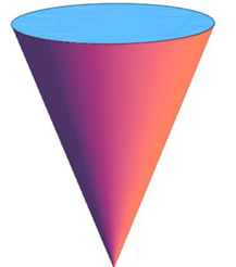
An inverted circular cone with a height 6 ft and base radius 2 ft is filled with water to a depth of 4 ft, see Figure 9.13. Find the work needed to pump all the water to the top of the conical tank. The density of water is 62.4 lb/ft³.

Figure 9.13: A conical water tank of height 6ft, base diameter 4ft, filled with water to a depth of 4ft

Figure 9.13: A conical water tank of height 6ft, base diameter 4ft, filled with water to a depth of 4ft.
Solution

Imagine inserting a vertical number line through the vertex of the cone with the origin at the top of the conical tank. Since the water is 4 ft deep, the water marks on the number line will lie on the interval [2,6][2,6]. Subdivide [2,6][2,6] into nn subintervals [yi−1,yi][y_{i-1},y_i] of equal width Δy\Delta y. The volume of water in the depth [yi−1,yi][y_{i-1},y_i] can be approximated by a circular disk DiD_i of height Δy\Delta y and radius rir_i. In Figure 9.14, we see similar triangles and consequently.

ri6−yi=26\frac{r_i}{6-y_i} = \frac{2}{6}

ri=26(6−yi)r_i = \frac{2}{6}(6-y_i)

Figure 9.14: Similar triangle

Figure 9.14: Similar triangle

Then the volume ViV_i of disk DiD_i is,

Vi=πr2Δy=π9(6−yi)2ΔyV_i = \pi r^2\Delta y = \frac{\pi}{9}(6-y_i)^2\Delta y

and using the density of water we find that the weight FiF_i of disk DiD_i is,

Fi=62.4Vi=62.4π9(6−yi)2ΔyF_i = 62.4V_i = \frac{62.4\pi}{9}(6-y_i)^2\Delta y

Then the work WiW_i needed to pump disk DiD_i to the top of the tank is approximately,

Wi≈(force)(distance)=Fiyi=62.4π9yi(6−yi)2ΔyW_i \approx (force)(distance) = F_iy_i = \frac{62.4\pi}{9}y_i(6-y_i)^2\Delta y

Applying the limit process, we find that the total work needed to pump the water to the top of the conical tank is,

(Work)=lim⁡Δy→0∑i=1n62.4π9yi(6−yi)2Δy=∫2662.4π9y(6−y)2 dy=∫2662.4π9(y3−12y2+36y) dy(Work)=6656π15 ft-lb≈1394 ft-lb.\begin{aligned} (Work) &= \lim_{\Delta y \to 0}\sum_{i=1}^{n}\frac{62.4\pi}{9}y_i(6-y_i)^2\Delta y \\ &= \int_2^6\frac{62.4\pi}{9}y(6-y)^2\,dy \\ &= \int_2^6\frac{62.4\pi}{9}(y^3-12y^2+36y)\,dy \\ (Work) &= \frac{6656\pi}{15}\ \text{ft-lb} \approx 1394\ \text{ft-lb.} \end{aligned}

9.5 Moments and Centres of Mass​

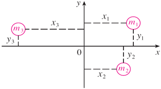
Suppose a beam is ll meters long, and that there are two weights on the beam: a m1m_1 kilogram weight d1d_1 meters from the fulcrum, another m2m_2 kilogram weight d2d_2 meters from the fulcrum end as in Figure 9.15. Where a fulcrum should be placed so that the beam balances? Let's assign a scale to the beam, from 0 at the left end to 10 at the right, so that we can denote locations on the beam simply as xx coordinates; the weights are at x=3x = 3, x=6x = 6, and x=8x = 8, as in Figure 9.15.

Figure 9.15: A beam with two masses

Figure 9.15: A beam with two masses.

Two masses m1m_1 and m2m_2 are attached to a rod of negligible mass on opposite sides of a fulcrum and at distances d1d_1 and d2d_2 from the fulcrum. The rod will balance if m1d1=m2d2m_1d_1 = m_2d_2.

Considering the following Figure 9.16, we can find out the position fulcrum.

Figure 9.16

Figure 9.16
  • suppose that the rod lies along the xx-axis with m1m_1 at x1x_1 and m2m_2 at x2x_2 and the center of mass at xˉ\bar{x}
  • Compare with the previous figure,

d1=xˉ−x1andd2=x2−xˉd_1 = \bar{x}-x_1 \quad \text{and} \quad d_2 = x_2-\bar{x}

  • Thus,
m1(xˉ−x1)=m2(x2−xˉ)m1xˉ+m2xˉ=m1x1+m2x2xˉ=m1x1+m2x2m1+m2\begin{aligned} m_1(\bar{x}-x_1) &= m_2(x_2-\bar{x}) \\ m_1\bar{x}+m_2\bar{x} &= m_1x_1+m_2x_2 \\ \bar{x} &= \frac{m_1x_1+m_2x_2}{m_1+m_2} \end{aligned}
  • In general, for a system with nn particles with the mass of each particle m1,m2…,mnm_1, m_2 \dots, m_n located at points x1,x2…,xnx_1, x_2 \dots, x_n on the xx-axis,

xˉ=∑i=1nmixi∑i=1nmi\bar{x} = \frac{\sum_{i=1}^{n}m_ix_i}{\sum_{i=1}^{n}m_i}

  • If we let m=∑i=1nmim = \sum_{i=1}^{n}m_i and the sum of individual moments M=∑i=1nmixiM = \sum_{i=1}^{n}m_ix_i, we obtain

mxˉ=Mm\bar{x} = M

We can consider another system, like Figure 9.17 below.

Figure 9.17

Figure 9.17
  • consider a system of nn particles with masses m1,m2…,mnm_1, m_2 \dots, m_n located at the points (x1,y1),(x2,y2),…,(xn,yn)(x_1,y_1), (x_2,y_2), \dots, (x_n,y_n) in the xyxy-plane
  • By analogy with the one-dimensional case, we define the moment of the system about the y-axis to be,

My=∑i=1nmixiM_y = \sum_{i=1}^{n}m_ix_i

and the moment of the system about the x-axis as,

Mx=∑i=1nmiyiM_x = \sum_{i=1}^{n}m_iy_i

  • the coordinates (xˉ,yˉ)(\bar{x},\bar{y}) of the center of mass are given in terms of the moments by the formulas,

xˉ=Mymandyˉ=Mxm\bar{x} = \frac{M_y}{m} \quad \text{and} \quad \bar{y} = \frac{M_x}{m}

  • the center of mass (xˉ,yˉ)(\bar{x},\bar{y}) is the point where a single particle of mass mm would have the same moments as the system

Example 9.14​

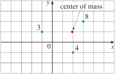
Find the moments and centre of mass of the system of objects that have masses 3, 4, and 8 at the points (−1,1)(-1,1), (2,−1)(2,-1), and (3,2)(3,2), respectively.

Figure 9.18

Figure 9.18
  • Calculate the moments about xx- and yy-axes from the formula MxM_x and MyM_y
  • Calculate the coordinate for the centre of mass (xˉ,yˉ)(\bar{x},\bar{y}) from the formula xˉ=Mym\bar{x} = \dfrac{M_y}{m} and yˉ=Mxm\bar{y} = \dfrac{M_x}{m}
Solution

The system of 3 particles with masses 3, 4 and 8 located at the points (−1,1)(-1,1), (2,−1)(2,-1), and (3,2)(3,2), respectively, in the xyxy-plane.

The moment of the system about the x-axis as,

Mx=∑i=1nmiyi=(3×1+4×(−1)+8×2)=15M_x = \sum_{i=1}^{n}m_iy_i = (3 \times 1 + 4 \times (-1) + 8 \times 2) = 15

The moment of the system about the y-axis to be,

My=∑i=1nmixi=(3×(−1)+4×2+8×3)=29M_y = \sum_{i=1}^{n}m_ix_i = (3 \times (-1) + 4 \times 2 + 8 \times 3) = 29

The center of mass (xˉ,yˉ)(\bar{x},\bar{y}) from the formula xˉ=Mym\bar{x} = \dfrac{M_y}{m} and yˉ=Mxm\bar{y} = \dfrac{M_x}{m}

xˉ=Mym=29(3+4+8)=1.93\bar{x} = \frac{M_y}{m} = \frac{29}{(3+4+8)} = 1.93

yˉ=Mxm=15(3+4+8)=1.0\bar{y} = \frac{M_x}{m} = \frac{15}{(3+4+8)} = 1.0

The center of mass (xˉ,yˉ)=(1.93,1)(\bar{x},\bar{y}) = (1.93, 1)

Example 9.15 (Centroid of a Lamina)​

  • What about the center of mass of a flat plate (lamina) that occupies the region R\mathcal{R} on a plane?
  • The center of mass of the plate is called the centroid of R\mathcal{R}
  • Use the symmetry principle: if R\mathcal{R} is symmetric about a line ll, then the centroid of R\mathcal{R} lies on ll
  • Example: what is the centroid of a rectangle?

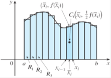
The region R between x = a and x = b under the graph of y = f(x)

  • Next, define moments such that if the entire mass of a region is concentrated at the center of mass, its moments remain unchanged.
  • Suppose that the region R\mathcal{R} lies between the lines x=ax = a and x=bx = b, above the xx-axis, and beneath the graph of ff, where ff is a continuous function
  • divide the interval [a,b][a,b] into nn subintervals with endpoints x0x_0, x1x_1, …\dots, xnx_n and equal width Δx\Delta x
  • choose the sample point xi∗x_i^* to be the midpoint xˉi\bar{x}_i of the iith subinterval, that is, xˉi=(xi−1+xi)/2\bar{x}_i = (x_{i-1}+x_i)/2
  • The centroid of the iith approximating rectangle RiR_i is its center Ci(xˉi,12f(xˉi))C_i\left(\bar{x}_i, \dfrac{1}{2}f(\bar{x}_i)\right). Its area is f(xˉi)Δxf(\bar{x}_i)\Delta x.

The region R approximated by rectangles, with the centroid of the i-th rectangle marked

  • The mass of the lamina is thus ρf(xˉi)Δx\rho f(\bar{x}_i)\Delta x
  • The moment of RiR_i about the yy-axis is the product of its mass and the distance from CiC_i to the yy-axis, i.e. xˉi\bar{x}_i. Thus,

My(Ri)=[ρf(xˉi)Δx]xˉi=ρxˉif(xˉi)ΔxM_y(R_i) = [\rho f(\bar{x}_i)\Delta x]\bar{x}_i = \rho\bar{x}_if(\bar{x}_i)\Delta x

  • Adding these moments, we obtain the moment of the polygonal approximation to RR
  • By taking the limit as n→∞n \to \infty, we obtain the moment of RR about the yy-axis,

My=lim⁡n→∞∑i=1nρxˉif(xˉi)Δx=ρ∫abxf(x) dxM_y = \lim_{n \to \infty}\sum_{i=1}^{n}\rho\bar{x}_if(\bar{x}_i)\Delta x = \rho\int_a^b xf(x)\,dx

  • Similarly, we compute the moment of RiR_i about the xx-axis as the product of its mass and the distance from CiC_i to the xx-axis:

Mx(Ri)=[ρf(xˉi)Δx]12f(xˉi)=ρ⋅12[f(xˉi)]2ΔxM_x(R_i) = [\rho f(\bar{x}_i)\Delta x]\frac{1}{2}f(\bar{x}_i) = \rho \cdot \frac{1}{2}[f(\bar{x}_i)]^2\Delta x

  • Adding the moments and take the limit to obtain the moment of RR about the xx-axis:

Mx=lim⁡n→∞∑i=1nρ⋅12[f(xˉi)]2Δx=ρ∫ab12[f(x)]2 dxM_x = \lim_{n \to \infty}\sum_{i=1}^{n}\rho \cdot \frac{1}{2}[f(\bar{x}_i)]^2\Delta x = \rho\int_a^b \frac{1}{2}[f(x)]^2\,dx

Recall the center of mass for a system of particles:

xˉ=Mymandyˉ=Mxm\bar{x} = \frac{M_y}{m} \quad \text{and} \quad \bar{y} = \frac{M_x}{m}

For a plate, the mass is

m=ρA=ρ∫abf(x) dxm = \rho A = \rho\int_a^b f(x)\,dx

Thus,

xˉ=Mym=ρ∫abxf(x) dxρ∫abf(x) dx=∫abxf(x) dx∫abf(x) dx=1A∫abxf(x) dx\bar{x} = \frac{M_y}{m} = \frac{\rho\int_a^b xf(x)\,dx}{\rho\int_a^b f(x)\,dx} = \frac{\int_a^b xf(x)\,dx}{\int_a^b f(x)\,dx} = \frac{1}{A}\int_a^b xf(x)\,dx

yˉ=Mxm=ρ∫ab12[f(x)]2dxρ∫abf(x) dx=∫ab12[f(x)]2dx∫abf(x) dx=1A∫ab12[f(x)]2dx\bar{y} = \frac{M_x}{m} = \frac{\rho\int_a^b \frac{1}{2}[f(x)]^2dx}{\rho\int_a^b f(x)\,dx} = \frac{\int_a^b \frac{1}{2}[f(x)]^2dx}{\int_a^b f(x)\,dx} = \frac{1}{A}\int_a^b \frac{1}{2}[f(x)]^2dx

9.6 Arc Length​

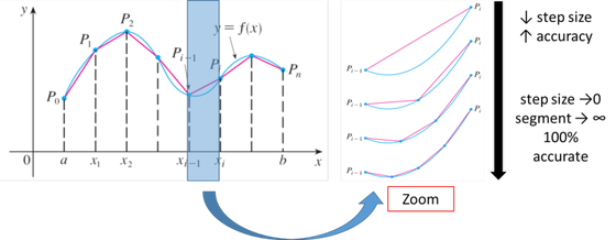
Let consider the following arc,

Figure 9.19

Figure 9.19

We want to determine the length of the continuous function y=f(x)y=f(x) on the interval [a,b][a,b]. We'll also need to assume that the derivative is continuous on [a,b][a,b].

Initially we'll need to estimate the length of the curve. We'll do this by dividing the interval up into nn equal subintervals each of width Δx\Delta x and we'll denote the point on the curve at each point by PiP_i. We can then approximate the curve by a series of straight lines connecting the points.

Now denote the length of each of these line segments by ∣Pi−1,Pi∣|P_{i-1},P_i| and the length of the curve will then be approximately,

L≈∑i=1n∣Pi−1−Pi∣L \approx \sum_{i=1}^{n}|P_{i-1}-P_i|

And we can get the exact length by taking nn larger and larger, towards infinity. In other words, the exact length will be,

L=lim⁡n→∞∑i=1n∣Pi−1−Pi∣L = \lim_{n \to \infty}\sum_{i=1}^{n}|P_{i-1}-P_i|

Now, let's get a better grasp on the length of each of these line segments. First, on each segment let's define,

Δyi=yi−yi−1=f(xi)−f(xi−1)\Delta y_i = y_i - y_{i-1} = f(x_i)-f(x_{i-1})

We can then compute directly the length of the line segments as follows:

∣Pi−1Pi∣=(xi−xi−1)2+(yi−yi−1)2=Δx2+Δyi2|P_{i-1}P_i| = \sqrt{(x_i-x_{i-1})^2+(y_i-y_{i-1})^2} = \sqrt{\Delta x^2+\Delta y_i^2}

∣Pi−Pi−1∣=(1+(f′(x∗))2)Δxor,=(1+(1f′(x∗))2)Δy|P_i-P_{i-1}| = \left(\sqrt{1+(f'(x^*))^2}\right)\Delta x \qquad or, = \left(\sqrt{1+\left(\frac{1}{f'(x^*)}\right)^2}\right)\Delta y

The exact length of the curve is then,

L=lim⁡n→∞∑i=1n∣Pi−1Pi∣=lim⁡n→∞∑i=1n1+[f′(xi∗)]2 Δx\begin{aligned} L &= \lim_{n \to \infty}\sum_{i=1}^{n}|P_{i-1}P_i| \\ &= \lim_{n \to \infty}\sum_{i=1}^{n}\sqrt{1+[f'(x_i^*)]^2}\ \Delta x \end{aligned}

However, using the definition of the definite integral, this is nothing more than,

L=∫ab1+[f′(x)]2 dxL = \int_a^b \sqrt{1+[f'(x)]^2}\,dx

A slightly more convenient notation (in our opinion anyway) is the following.

L=∫ab1+(dydx)2 dxL = \int_a^b \sqrt{1+\left(\frac{dy}{dx}\right)^2}\,dx

In a similar fashion we can also derive a formula for x=h(y)x=h(y) on [c,d][c,d]. This formula is,

L=∫cd1+[h′(y)]2 dy=∫cd1+(dxdy)2 dyL = \int_c^d \sqrt{1+[h'(y)]^2}\,dy = \int_c^d \sqrt{1+\left(\frac{dx}{dy}\right)^2}\,dy

Example 9.16​

Find the length of the arc, y=x33+14xy = \dfrac{x^3}{3}+\dfrac{1}{4x}, 1≤x≤21 \le x \le 2 as shown in Figure 9.20

Figure 9.20

Figure 9.20
Solution

The derivative is,

dydx=x2−14x2\frac{dy}{dx} = x^2-\frac{1}{4x^2}

We calculate a perfect square as follows:

1+(dydx)2=1+(x4−12+116x4)=x4+12+116x4=(x2+14x2)2=x2+14x2\begin{aligned} \sqrt{1+\left(\frac{dy}{dx}\right)^2} &= \sqrt{1+\left(x^4-\frac{1}{2}+\frac{1}{16x^4}\right)} \\ &= \sqrt{x^4+\frac{1}{2}+\frac{1}{16x^4}} \\ &= \sqrt{\left(x^2+\frac{1}{4x^2}\right)^2} = x^2+\frac{1}{4x^2} \end{aligned}

Then we obtain,

(Arc length)=∫121+[f′(x)]2 dx=∫12(x2+14x2)dx=x33−14x∣12=5924\begin{aligned} (Arc\ length) &= \int_1^2\sqrt{1+[f'(x)]^2}\,dx = \int_1^2\left(x^2+\frac{1}{4x^2}\right)dx \\ &= \frac{x^3}{3}-\frac{1}{4x}\Big|_1^2 \\ &= \frac{59}{24} \end{aligned}

Example 9.17​

Find the arc length of f(x)=x28−ln⁡xf(x) = \dfrac{x^2}{8}-\ln x, 1≤x≤e1 \le x \le e as shown in Figure 9.21

Figure 9.21

Figure 9.21
Solution

The derivative is,

dydx=x4−1x\frac{dy}{dx} = \frac{x}{4}-\frac{1}{x}

The integrand of the arc length integral is given by,

1+(f′(x))2=1+(x216−12+1x2)=x216+12+1x2=(x4+1x)2=x4+1xsince x>0\begin{aligned} \sqrt{1+(f'(x))^2} &= \sqrt{1+\left(\frac{x^2}{16}-\frac{1}{2}+\frac{1}{x^2}\right)} \\ &= \sqrt{\frac{x^2}{16}+\frac{1}{2}+\frac{1}{x^2}} \\ &= \sqrt{\left(\frac{x}{4}+\frac{1}{x}\right)^2} \\ &= \frac{x}{4}+\frac{1}{x} \qquad \text{since } x > 0 \end{aligned}

Then we find,

(Arc length)=∫1e1+[f′(x)]2 dx=∫1e(x4+1x)dx=x28+ln⁡x∣1e=e2+78\begin{aligned} (Arc\ length) &= \int_1^e\sqrt{1+[f'(x)]^2}\,dx = \int_1^e\left(\frac{x}{4}+\frac{1}{x}\right)dx \\ &= \frac{x^2}{8}+\ln x\Big|_1^e \\ &= \frac{e^2+7}{8} \end{aligned}

9.7 The Area of a Surface of Revolution​

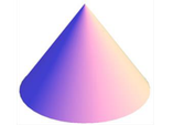
Let CC be a right circular cone with a base radius of rr and slant height hh, see Figure 9.22. If we slice open the cone at its vertex along a slant height and lay it on a plane, we obtain a sector of a circle of radius hh and an intercepted arc of length 2πr2\pi r. Then the central angle θ\theta of the sector satisfies:

Figure 9.22: A right circular cone with slant height &quot;h&quot; and radius &quot;r&quot;

Figure 9.22: A right circular cone with slant height "h" and radius "r".

hθ=2πrh\theta = 2\pi r

Consequently, the area of the sector (or equivalently the surface area of CC) is,

(Surface area of a cone)=θ2h2=πrh(9.4)(Surface\ area\ of\ a\ cone) = \frac{\theta}{2}h^2 = \pi rh \qquad (9.4)

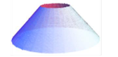
Next, consider a frustum of a cone with radii r2>r1r_2 > r_1 and slant height ll, see Figure 9.23. Using similar right triangles, as shown in Figure 9.24, where,

Figure 9.23: A frustum of cone with radii r2 &gt; r1 and slant height &quot;l&quot;

Figure 9.23: A frustum of cone with radii r2 > r1 and slant height "l".

l=l2−l1l = l_2-l_1

We get,

l2r2=l1r1\frac{l_2}{r_2} = \frac{l_1}{r_1}

Figure 9.24: Similar triangles where AB = l1, AC = l2

Figure 9.24: Similar triangles where AB = l1, AC = l2

Note, the surface area of a frustum is the difference of the surface areas of two cones. Applying formula (9.4), we obtain,

(Surface area of a frustum)=πr2l2−πr1l1=π(r2l2−r1l1)=π(r2+r1)(l2−l1)Since r1l2−r2l1=0=2πrl.where r=r1+r22\begin{aligned} (Surface\ area\ of\ a\ frustum) &= \pi r_2l_2-\pi r_1l_1 = \pi(r_2l_2-r_1l_1) \\ &= \pi(r_2+r_1)(l_2-l_1) \qquad \text{Since } r_1l_2-r_2l_1 = 0 \\ &= 2\pi rl. \qquad \text{where } r = \frac{r_1+r_2}{2} \end{aligned}

Example 9.18​

Compute the surface area of a sphere of radius rr. The sphere can be obtained by rotating the graph of f(x)=r2−x2f(x) = \sqrt{r^2-x^2} about the xx-axis.

Solution

The derivative f′f' is −x/r2−x2-x/\sqrt{r^2-x^2}, so the surface area is given by,

A=2π∫−rrr2−x21+x2r2−x2 dx=2π∫−rrr2−x2r2r2−x2 dx=2π∫−rrr dx=2πr∫−rr1 dx=4πr2\begin{aligned} A &= 2\pi\int_{-r}^{r}\sqrt{r^2-x^2}\sqrt{1+\frac{x^2}{r^2-x^2}}\,dx \\ &= 2\pi\int_{-r}^{r}\sqrt{r^2-x^2}\sqrt{\frac{r^2}{r^2-x^2}}\,dx \\ &= 2\pi\int_{-r}^{r}r\,dx = 2\pi r\int_{-r}^{r}1\,dx = 4\pi r^2 \end{aligned}

If the curve is rotated around the yy axis, the formula is nearly identical, because the length of the line segment we use to approximate a portion of the curve doesn't change. Instead of the radius f(xi∗)f(x_i^*), we use the new radius xˉi=(xi+xi+1)/2\bar{x}_i = (x_i+x_{i+1})/2, and the surface area integral becomes,

∫ab2πx1+(f′(x))2 dx.\int_a^b 2\pi x\sqrt{1+(f'(x))^2}\,dx.

Example 9.19​

Compute the area of the surface formed when f(x)=x2f(x) = x^2 between 0 and 2 is rotated around the yy-axis.

Solution

We compute f′(x)=2xf'(x) = 2x, and then,

2π∫02x1+4x2 dx=π6(173/2−1)2\pi\int_0^2 x\sqrt{1+4x^2}\,dx = \frac{\pi}{6}(17^{3/2}-1)

by a simple substitution.