KIX1001 2020/2021 Semester 1 — Paper 2

Original Question Paper (PDF)

Paper details

Academic session 2020/2021, Semester 1 · Open Book Exam #2 out of 2 · 2 questions (Question 3 and Question 4), each printed in 10 sets · 21 printed pages.

Students answered only the set matching the last digit of their matrix number:

Last digit of matrix number	Set	Pages
1	Set #1	2–3
2	Set #2	4–5
3	Set #3	6–7
4	Set #4	8–9
5	Set #5	10–11
6	Set #6	12–13
7	Set #7	14–15
8	Set #8	16–17
9	Set #9	18–19
0	Set #10	20–21

All ten sets share the same structure — a low-pass LRC filter in Question 3 and a Maclaurin/power-series problem in Question 4 — and differ only in the numbers (the noise frequency in $V_{input}$ and the constant inside the logarithm).

Questions are reproduced in English from the bilingual original. Solutions are worked in full.

Figures and part letters

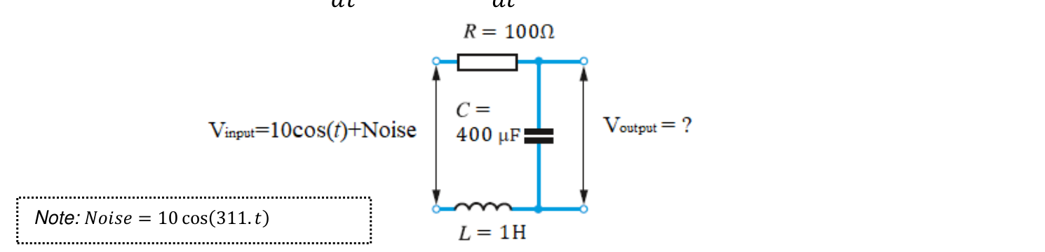
Question 3's circuit figure is shared by all ten sets; Figure Q3(a) as printed for Set #1 is reproduced below. (The question stem refers to "Figure Q3(b)", but only Figure Q3(a) is printed anywhere in the 21 pages — a slip in the original paper.)

The part letters of Question 3 run continuously across the sets — Set #1 prints (a), (b); Set #2 prints (c), (d); … Set #10 prints (s), (t) — and the solutions below reproduce the letters exactly as printed. Question 4 is lettered (a) and (b) in every set.

No initial conditions are printed anywhere in this paper, so each Question 3 solution assumes the circuit starts at rest, $V_{output}(0) = V_{output}'(0) = 0$; only the two arbitrary constants change under other initial conditions.

Reference only — these are not official answers

These solutions are revision aids, not examiner answers. They were produced with the help of a large language model and then checked, but an LLM can still be wrong: expect the occasional arithmetic slip, a different method than your lecturer's, or a misreading of the printed question. The question wording is reproduced by hand from a scan of the original paper, so it too may differ in small ways from what was printed.

Use this page as a worked suggestion to check, not as ground truth. Always compare against the original paper (linked above) and your own lecture notes, and if something here disagrees with your lecturer, trust your lecturer. Marks shown are the paper's allocations, not a marking scheme.

Set #1 (last matrix digit 1)

Question 3 (Set #1)

Question

Given the governing equation of the low pass filter with LRC circuit, where the inductance ($L = 1$ H), resistance ($R = 100\ \Omega$), and capacitance ($C = 0.0004$ F) are shown in Figure Q3(b) of the original paper:

$$LC\frac{d^2V_{output}}{dt^2} + RC\frac{dV_{output}}{dt} + V_{output} = V_{input}$$

The shared circuit diagram (Figure Q3(a) in the original paper — the stem's reference to "Figure Q3(b)" is a printing slip, as only Figure Q3(a) is printed) shows a series LRC low-pass filter driven by a source $V_{input} = 10\cos(t) + \text{Noise}$, with $R = 100\ \Omega$, $C = 400\ \mu$F, $L = 1$ H and the output $V_{output}$ taken across the capacitor; see Figure Q3(a) in the original paper.

You are designing the circuit to obtain output voltage, $V_{output}$ by reducing/removing the high frequency noise only from the input voltage, $V_{input}$. $V_{input}$ for time, $t > 0$ is given as:

$$V_{input} = 10\cos(t) + 10\cos(311t)$$

Note: $\text{Noise} = 10\cos(311t)$.

Question 3(a) (13 marks)

Question

Find the total output voltage, $V_{output}$ for time, $t > 0$. Use the trigonometric function (sine & cosine functions) to solve the non-homogeneous part.

Solution

Technique. A second-order linear ODE with constant coefficients is solved in two stages: the complementary function from the auxiliary (characteristic) equation, then a particular integral for each driving tone by the method of undetermined coefficients using a sine/cosine trial function.

Step 1 — Substitute the component values.

With $L = 1$ H, $R = 100\ \Omega$ and $C = 0.0004$ F,

$$LC = (1)(0.0004) = 0.0004, \qquad RC = (100)(0.0004) = 0.04,$$

so the governing equation is

$$0.0004\,\frac{d^2V_{output}}{dt^2} + 0.04\,\frac{dV_{output}}{dt} + V_{output} = V_{input}(t).$$

Step 2 — Complementary function (homogeneous part).

Try $V_{output} = e^{rt}$. Then

$$0.0004r^2 + 0.04r + 1 = 0 \;\Longrightarrow\; r^2 + 100r + 2500 = 0 \;\Longrightarrow\; (r+50)^2 = 0,$$

so $r = -50$ is a repeated root. Hence

$$V_{c}(t) = (A + Bt)e^{-50t}.$$

Step 3 — Particular integral for the wanted signal $10\cos t$.

Try $V_{p1} = a\cos t + b\sin t$, so that $V_{p1}' = -a\sin t + b\cos t$ and $V_{p1}'' = -a\cos t - b\sin t$. Substituting into the ODE and collecting the $\cos t$ and $\sin t$ terms:

$$(-0.0004a + 0.04b + a)\cos t + (-0.0004b - 0.04a + b)\sin t = 10\cos t,$$$$\cos t:\; 0.9996a + 0.04b = 10, \qquad \sin t:\; -0.04a + 0.9996b = 0.$$

From the second equation

$$b = \frac{0.04}{0.9996}\,a = \frac{100}{2499}\,a .$$

Substituting into the first equation, and writing $0.9996 = \frac{2499}{2500}$ and $0.04 = \frac{1}{25}$,

$$a\left(\frac{2499}{2500} + \frac{4}{2499}\right) = 10 \;\Longrightarrow\; a\cdot\frac{6255001}{6247500} = 10 \;\Longrightarrow\; a = \frac{62475000}{6255001} \approx 9.9880,$$$$b = \frac{100}{2499}\,a = \frac{2500000}{6255001} \approx 0.39968 .$$

Therefore

$$V_{p1} = 9.9880\cos t + 0.39968\sin t .$$

Step 4 — Particular integral for the noise $10\cos(311t)$.

Try $V_{p2} = c\cos 311t + d\sin 311t$. With $\omega = 311$ rad/s, $\omega^2 = 96721$, so $V_{p2}'' = -96721\,V_{p2}$ and $V_{p2}' = 311(-c\sin 311t + d\cos 311t)$. Substituting:

$$(1 - 0.0004(96721))c + 0.04(311)d = 10, \qquad -0.04(311)c + (1 - 0.0004(96721))d = 0,$$$$-37.6884\,c + 12.44\,d = 10, \qquad -37.6884\,d - 12.44\,c = 0 .$$

From the second equation $d = -\frac{12.44}{37.6884}\,c = -0.33008\,c$. Substituting into the first:

$$-37.6884c + 12.44(-0.33008c) = 10 \;\Longrightarrow\; -41.7945\,c = 10 \;\Longrightarrow\; c = -0.23927,$$$$d = -0.33008(-0.23927) = 0.078976 .$$

So

$$V_{p2} = -0.23927\cos 311t + 0.078976\sin 311t$$

(exactly, $c = -\frac{2355525000}{9844806841}$ and $d = \frac{777500000}{9844806841}$).

Step 5 — Total solution.

Add the complementary function and both particular integrals:

$$V_{output}(t) = (A + Bt)e^{-50t} + 9.9880\cos t + 0.39968\sin t - 0.23927\cos 311t + 0.078976\sin 311t .$$

note

Question 3 prints no initial conditions, so $A$ and $B$ are arbitrary constants and the expression above is the complete general solution for $t > 0$. If the usual "circuit initially at rest" assumption $V_{output}(0) = V_{output}'(0) = 0$ is imposed, then $A = -9.7487$ and $B = -512.40$, giving

$$V_{output}(t) = (-9.7487 - 512.40t)e^{-50t} + 9.9880\cos t + 0.39968\sin t - 0.23927\cos 311t + 0.078976\sin 311t .$$

Answer: $V_{output}(t) = (A + Bt)e^{-50t} + 9.9880\cos t + 0.39968\sin t - 0.23927\cos 311t + 0.078976\sin 311t$ V for $t > 0$ (with $A$, $B$ arbitrary; $A = -9.7487$, $B = -512.40$ if the circuit starts from rest).

---

Question 3(b) (2 marks)

Question

Refer to the steady state result of $V_{output}$ only, check if the noise is successfully reduced/removed ($> 90\%$ amplitude reduction) or not. Hint: amplitude $= \sqrt{a^2 + b^2}$ for $a\cos(\omega t) + b\sin(\omega t)$ function.

Solution

Technique. The steady state is the particular integral alone: the transient $(A + Bt)e^{-50t}$ decays to zero because $r = -50 < 0$. Each steady tone has the form $a\cos\omega t + b\sin\omega t$, whose amplitude is $\sqrt{a^2+b^2}$.

Wanted signal ($\omega = 1$ rad/s). With $a = 9.9880$, $b = 0.39968$:

$$A_{1} = \sqrt{9.9880^2 + 0.39968^2} = \sqrt{99.760 + 0.1597} = \sqrt{99.920} = 9.9960 .$$

Noise ($\omega = 311$ rad/s). With $c = -0.23927$, $d = 0.078976$:

$$A_{311} = \sqrt{(-0.23927)^2 + (0.078976)^2} = \sqrt{0.057248 + 0.006237} = \sqrt{0.063485} = 0.251963 .$$

Amplitude reduction of the noise.

$$\text{reduction} = \frac{10 - 0.251963}{10}\times 100\% = 97.48\% .$$

Since $97.48\% > 90\%$, the high-frequency noise is successfully reduced — only about 2.5% of its amplitude survives. The wanted signal is passed almost untouched (9.9960 out of 10, a 0.04% loss), which is exactly what a low-pass filter should do.

Short cut: for a single tone of frequency $\omega$ the steady amplitude is $\frac{10}{\sqrt{(1-0.0004\omega^2)^2 + (0.04\omega)^2}}$, which gives $\frac{10}{\sqrt{37.6884^2 + 12.44^2}} = \frac{10}{39.6884} = 0.251963$ for $\omega = 311$.

Answer: Noise amplitude $= 0.2520$ V (exactly $\frac{25000}{99221}$ V) against 10 V at the input — a $97.48\%$ reduction, so yes, the noise is successfully reduced ($> 90\%$).

---

Question 4 (Set #1)

Parts (a) and (b) are independent statements; part (b) uses the expansion obtained in part (a).

Question 4(a) (4 marks)

Question

Find the power series until the $x^5$ term for the following function

$$f(x) = \ln(5+x)$$

using the Maclaurin's Series given below

$$f(x) = f(0) + xf'(0) + \frac{x^2}{2!}f''(0) + \frac{x^3}{3!}f'''(0) + \cdots$$

Solution

Technique. Compute the successive derivatives of $f$, evaluate each at $x = 0$, and divide the $n$-th derivative by $n!$ to get the coefficient of $x^n$.

$$f(x) = \ln(5+x), \qquad f'(x) = \frac{1}{5+x}, \qquad f''(x) = -\frac{1}{(5+x)^2},$$$$f'''(x) = \frac{2}{(5+x)^3}, \qquad f^{(4)}(x) = -\frac{6}{(5+x)^4}, \qquad f^{(5)}(x) = \frac{24}{(5+x)^5}.$$

At $x = 0$:

$n$	$f^{(n)}(x)$	$f^{(n)}(0)$	term $\frac{x^n}{n!}f^{(n)}(0)$
0	$\ln(5+x)$	$\ln 5$	$\ln 5$
1	$(5+x)^{-1}$	$1/5$	$x/5$
2	$-(5+x)^{-2}$	$-1/25$	$-x^2/50$
3	$2(5+x)^{-3}$	$2/125$	$x^3/375$
4	$-6(5+x)^{-4}$	$-6/625$	$-x^4/2500$
5	$24(5+x)^{-5}$	$24/3125$	$x^5/15625$

Substituting into the Maclaurin series:

$$f(x) = \ln 5 + \frac{x}{5} - \frac{x^2}{2\cdot 25} + \frac{2x^3}{6\cdot 125} - \frac{6x^4}{24\cdot 625} + \frac{24x^5}{120\cdot 3125} + \cdots$$$$f(x) = \ln 5 + \frac{x}{5} - \frac{x^2}{50} + \frac{x^3}{375} - \frac{x^4}{2500} + \frac{x^5}{15625} + \cdots$$

Check (standard-series route). $\ln(5+x) = \ln 5 + \ln\left(1 + \frac{x}{5}\right)$ and $\ln(1+u) = u - \frac{u^2}{2} + \frac{u^3}{3} - \frac{u^4}{4} + \frac{u^5}{5} - \cdots$ with $u = \frac{x}{5}$ gives exactly the same coefficients. The expansion is valid for $|x| < 5$.

Answer: $\ln(5+x) = \ln 5 + \frac{x}{5} - \frac{x^2}{50} + \frac{x^3}{375} - \frac{x^4}{2500} + \frac{x^5}{15625} + \cdots$

---

Question 4(b) (11 marks)

Question

Apply the power series method and part (a) to find the particular solution at $x = 0$ for the following differential equation:

$$y'' - 2xy = \ln(5+x), \qquad y(0) = y'(0) = 8$$

Solution

Technique. Assume a power-series solution $y = \sum_{n\ge0} a_n x^n$, substitute it into the ODE, and match coefficients of $x^k$. The initial conditions fix $a_0$ and $a_1$, and the part (a) expansion supplies the coefficients of the right-hand side.

Step 1 — Series for each term.

$$y = \sum_{n=0}^{\infty} a_n x^n, \qquad y'' = \sum_{n=2}^{\infty} n(n-1)a_n x^{n-2} = \sum_{k=0}^{\infty}(k+2)(k+1)a_{k+2}\,x^{k},$$$$2xy = \sum_{n=0}^{\infty} 2a_n x^{n+1} = \sum_{k=1}^{\infty} 2a_{k-1}\,x^{k}.$$

From part (a),

$$\ln(5+x) = \sum_{k=0}^{\infty} b_k x^k, \qquad b_0 = \ln 5,\; b_1 = \frac{1}{5},\; b_2 = -\frac{1}{50},\; b_3 = \frac{1}{375},\; b_4 = -\frac{1}{2500},\; b_5 = \frac{1}{15625}.$$

Step 2 — Initial conditions.

$$y(0) = a_0 = 8, \qquad y'(0) = a_1 = 8 .$$

Step 3 — Recurrence.

Substituting into $y'' - 2xy = \ln(5+x)$ and equating coefficients of $x^k$ (with $a_{-1} \equiv 0$):

$$(k+2)(k+1)a_{k+2} - 2a_{k-1} = b_k \qquad (k = 0, 1, 2, \dots).$$

Step 4 — Generate the coefficients.

$k$	equation	coefficient found
0	$2a_2 = \ln 5$	$a_2 = \frac{\ln 5}{2} \approx 0.80472$
1	$6a_3 = \frac{1}{5} + 2(8) = \frac{81}{5}$	$a_3 = \frac{27}{10} = 2.7$
2	$12a_4 = -\frac{1}{50} + 2(8) = \frac{799}{50}$	$a_4 = \frac{799}{600} \approx 1.3317$
3	$20a_5 = \frac{1}{375} + 2\left(\frac{\ln 5}{2}\right)$	$a_5 = \frac{1}{7500} + \frac{\ln 5}{20} \approx 0.080605$
4	$30a_6 = -\frac{1}{2500} + 2\left(\frac{27}{10}\right) = \frac{13499}{2500}$	$a_6 = \frac{13499}{75000} \approx 0.17999$
5	$42a_7 = \frac{1}{15625} + 2\left(\frac{799}{600}\right) = \frac{499387}{187500}$	$a_7 = \frac{71341}{1125000} \approx 0.063414$

Step 5 — Particular solution.

$$y(x) = 8 + 8x + \frac{\ln 5}{2}x^2 + \frac{27}{10}x^3 + \frac{799}{600}x^4 + \left(\frac{1}{7500} + \frac{\ln 5}{20}\right)x^5 + \frac{13499}{75000}x^6 + \frac{71341}{1125000}x^7 + \cdots$$

Numerically,

$$y(x) \approx 8 + 8x + 0.80472x^2 + 2.7x^3 + 1.3317x^4 + 0.080605x^5 + 0.17999x^6 + 0.063414x^7 + \cdots$$

Check. Differentiating term by term and substituting back gives $y'' - 2xy - \ln(5+x) = O(x^6)$, and $y(0) = 8$, $y'(0) = 8$ as required.

Answer: $y(x) = 8 + 8x + \frac{\ln 5}{2}x^2 + \frac{27}{10}x^3 + \frac{799}{600}x^4 + \left(\frac{1}{7500} + \frac{\ln 5}{20}\right)x^5 + \frac{13499}{75000}x^6 + \frac{71341}{1125000}x^7 + \cdots$

---

Set #2 (last matrix digit 2)

Question 3 (Set #2)

Question

Given the governing equation of the low pass filter with LRC circuit, where the inductance ($L = 1$ H), resistance ($R = 100\ \Omega$), and capacitance ($C = 0.0004$ F) are shown in Figure Q3(b) of the original paper:

$$LC\frac{d^2V_{output}}{dt^2} + RC\frac{dV_{output}}{dt} + V_{output} = V_{input}$$

The shared circuit diagram (Figure Q3(a) in the original paper — the stem's reference to "Figure Q3(b)" is a printing slip, as only Figure Q3(a) is printed) shows the same series LRC low-pass filter as Set #1: a source $V_{input} = 10\cos(t) + \text{Noise}$ in series with $R = 100\ \Omega$ and $L = 1$ H, with $C = 400\ \mu$F across the output $V_{output}$; see Figure Q3(a) in the original paper.

You are designing the circuit to obtain output voltage, $V_{output}$ by reducing/removing the high frequency noise only from the input voltage, $V_{input}$. $V_{input}$ for time, $t > 0$ is given as:

$$V_{input} = 10\cos(t) + 10\cos(322t)$$

Note: $\text{Noise} = 10\cos(322t)$.

Question 3(c) (13 marks)

Question

Find the total output voltage, $V_{output}$ for time, $t > 0$. Use the trigonometric function (sine & cosine functions) to solve the non-homogeneous part.

Solution

Technique. Solve the constant-coefficient linear ODE by (i) the auxiliary (characteristic) equation for the complementary function, then (ii) the method of undetermined coefficients with a sine/cosine trial for each of the two driving tones. Only the noise frequency changes from Set #1.

Step 1 — Substitute the component values.

With $L = 1$ H, $R = 100\ \Omega$ and $C = 0.0004$ F,

$$LC = 0.0004, \qquad RC = 0.04,$$

so

$$0.0004\,\frac{d^2V_{output}}{dt^2} + 0.04\,\frac{dV_{output}}{dt} + V_{output} = V_{input}(t).$$

Step 2 — Complementary function (homogeneous part).

With $V_{output} = e^{rt}$:

$$0.0004r^2 + 0.04r + 1 = 0 \;\Longrightarrow\; r^2 + 100r + 2500 = 0 \;\Longrightarrow\; (r+50)^2 = 0,$$

so $r = -50$ is a repeated root and

$$V_{c}(t) = (A + Bt)e^{-50t}.$$

Step 3 — Particular integral for the wanted signal $10\cos t$.

Try $V_{p1} = a\cos t + b\sin t$. Collecting $\cos t$ and $\sin t$:

$$\cos t:\; 0.9996a + 0.04b = 10, \qquad \sin t:\; -0.04a + 0.9996b = 0,$$

so $b = \frac{0.04}{0.9996}a = \frac{100}{2499}a$ and

$$a\left(\frac{2499}{2500} + \frac{4}{2499}\right) = 10 \;\Longrightarrow\; a = \frac{62475000}{6255001} \approx 9.9880, \qquad b = \frac{2500000}{6255001} \approx 0.39968 .$$

Therefore

$$V_{p1} = 9.9880\cos t + 0.39968\sin t .$$

Step 4 — Particular integral for the noise $10\cos(322t)$.

Try $V_{p2} = c\cos 322t + d\sin 322t$. Here $\omega = 322$ rad/s, $\omega^2 = 103684$, so $V_{p2}'' = -103684\,V_{p2}$ and $V_{p2}' = 322(-c\sin 322t + d\cos 322t)$. Substituting:

$$(1 - 0.0004(103684))c + 0.04(322)d = 10, \qquad -0.04(322)c + (1 - 0.0004(103684))d = 0,$$$$-40.4736\,c + 12.88\,d = 10, \qquad -40.4736\,d - 12.88\,c = 0 .$$

From the second equation $d = -\frac{12.88}{40.4736}\,c = -0.31823\,c$. Substituting into the first:

$$-40.4736c + 12.88(-0.31823c) = 10 \;\Longrightarrow\; -44.5724\,c = 10 \;\Longrightarrow\; c = -0.22435,$$$$d = -0.31823(-0.22435) = 0.071397 .$$

So

$$V_{p2} = -0.22435\cos 322t + 0.071397\sin 322t$$

(exactly, $c = -\frac{39525000}{176172529}$ and $d = \frac{12578125}{176172529}$).

Step 5 — Total solution.

$$V_{output}(t) = (A + Bt)e^{-50t} + 9.9880\cos t + 0.39968\sin t - 0.22435\cos 322t + 0.071397\sin 322t .$$

note

Question 3 prints no initial conditions, so $A$ and $B$ are arbitrary constants and the expression above is the complete general solution for $t > 0$. If the "circuit initially at rest" assumption $V_{output}(0) = V_{output}'(0) = 0$ is imposed, then $A = -9.7637$ and $B = -511.57$, giving

$$V_{output}(t) = (-9.7637 - 511.57t)e^{-50t} + 9.9880\cos t + 0.39968\sin t - 0.22435\cos 322t + 0.071397\sin 322t .$$

Answer: $V_{output}(t) = (A + Bt)e^{-50t} + 9.9880\cos t + 0.39968\sin t - 0.22435\cos 322t + 0.071397\sin 322t$ V for $t > 0$ (with $A$, $B$ arbitrary; $A = -9.7637$, $B = -511.57$ if the circuit starts from rest).

---

Question 3(d) (2 marks)

Question

Refer to the steady state result of $V_{output}$ only, check if the noise is successfully reduced/removed ($> 90\%$ amplitude reduction) or not. Hint: amplitude $= \sqrt{a^2 + b^2}$ for $a\cos(\omega t) + b\sin(\omega t)$ function.

Solution

Technique. The steady state is the particular integral alone (the $(A+Bt)e^{-50t}$ transient dies out since $r = -50 < 0$). Each steady tone $a\cos\omega t + b\sin\omega t$ has amplitude $\sqrt{a^2+b^2}$.

Wanted signal ($\omega = 1$ rad/s). With $a = 9.9880$, $b = 0.39968$:

$$A_{1} = \sqrt{9.9880^2 + 0.39968^2} = \sqrt{99.760 + 0.1597} = \sqrt{99.920} = 9.9960 .$$

Noise ($\omega = 322$ rad/s). With $c = -0.22435$, $d = 0.071397$:

$$A_{322} = \sqrt{(-0.22435)^2 + (0.071397)^2} = \sqrt{0.050335 + 0.005098} = \sqrt{0.055432} = 0.235440 .$$

Amplitude reduction of the noise.

$$\text{reduction} = \frac{10 - 0.235440}{10}\times 100\% = 97.65\% .$$

Since $97.65\% > 90\%$, the high-frequency noise is successfully reduced. The wanted signal passes almost untouched (9.9960 out of 10, a 0.04% loss).

Short cut: the steady amplitude of a single tone is $\frac{10}{\sqrt{(1-0.0004\omega^2)^2 + (0.04\omega)^2}}$; for $\omega = 322$ this is $\frac{10}{\sqrt{40.4736^2 + 12.88^2}} = \frac{10}{42.4736} = 0.235440$.

Answer: Noise amplitude $= 0.2354$ V (exactly $\frac{6250}{26546}$ V) against 10 V at the input — a $97.65\%$ reduction, so yes, the noise is successfully reduced ($> 90\%$).

---

Question 4 (Set #2)

Parts (a) and (b) are independent statements; part (b) uses the expansion obtained in part (a).

Question 4(a) (4 marks)

Question

Find the power series until the $x^5$ term for the following function

$$f(x) = \ln(10+x)$$

using the Maclaurin's Series given below

$$f(x) = f(0) + xf'(0) + \frac{x^2}{2!}f''(0) + \frac{x^3}{3!}f'''(0) + \cdots$$

Solution

Technique. Differentiate repeatedly, evaluate each derivative at $x = 0$, then divide the $n$-th derivative by $n!$ for the coefficient of $x^n$.

$$f(x) = \ln(10+x), \qquad f'(x) = \frac{1}{10+x}, \qquad f''(x) = -\frac{1}{(10+x)^2},$$$$f'''(x) = \frac{2}{(10+x)^3}, \qquad f^{(4)}(x) = -\frac{6}{(10+x)^4}, \qquad f^{(5)}(x) = \frac{24}{(10+x)^5}.$$

At $x = 0$:

$n$	$f^{(n)}(x)$	$f^{(n)}(0)$	term $\frac{x^n}{n!}f^{(n)}(0)$
0	$\ln(10+x)$	$\ln 10$	$\ln 10$
1	$(10+x)^{-1}$	$1/10$	$x/10$
2	$-(10+x)^{-2}$	$-1/100$	$-x^2/200$
3	$2(10+x)^{-3}$	$2/1000$	$x^3/3000$
4	$-6(10+x)^{-4}$	$-6/10000$	$-x^4/40000$
5	$24(10+x)^{-5}$	$24/100000$	$x^5/500000$

Substituting into the Maclaurin series:

$$f(x) = \ln 10 + \frac{x}{10} - \frac{x^2}{2\cdot 100} + \frac{2x^3}{6\cdot 1000} - \frac{6x^4}{24\cdot 10000} + \frac{24x^5}{120\cdot 100000} + \cdots$$$$f(x) = \ln 10 + \frac{x}{10} - \frac{x^2}{200} + \frac{x^3}{3000} - \frac{x^4}{40000} + \frac{x^5}{500000} + \cdots$$

Check (standard-series route). $\ln(10+x) = \ln 10 + \ln\left(1 + \frac{x}{10}\right)$ with $\ln(1+u) = u - \frac{u^2}{2} + \frac{u^3}{3} - \frac{u^4}{4} + \frac{u^5}{5} - \cdots$ and $u = \frac{x}{10}$ gives the same coefficients. The expansion is valid for $|x| < 10$.

Answer: $\ln(10+x) = \ln 10 + \frac{x}{10} - \frac{x^2}{200} + \frac{x^3}{3000} - \frac{x^4}{40000} + \frac{x^5}{500000} + \cdots$

---

Question 4(b) (11 marks)

Question

Apply the power series method and part (a) to find the particular solution at $x = 0$ for the following differential equation

$$y'' - 2xy = \ln(10+x), \qquad y(0) = y'(0) = 3$$

Solution

Technique. Assume $y = \sum_{n\ge0} a_n x^n$, substitute into the ODE and match coefficients of $x^k$. The initial conditions give $a_0$ and $a_1$; the part (a) expansion gives the right-hand-side coefficients.

Step 1 — Series for each term.

$$y = \sum_{n=0}^{\infty} a_n x^n, \qquad y'' = \sum_{n=2}^{\infty} n(n-1)a_n x^{n-2} = \sum_{k=0}^{\infty}(k+2)(k+1)a_{k+2}\,x^{k},$$$$2xy = \sum_{n=0}^{\infty} 2a_n x^{n+1} = \sum_{k=1}^{\infty} 2a_{k-1}\,x^{k}.$$

From part (a),

$$\ln(10+x) = \sum_{k=0}^{\infty} b_k x^k, \qquad b_0 = \ln 10,\; b_1 = \frac{1}{10},\; b_2 = -\frac{1}{200},\; b_3 = \frac{1}{3000},\; b_4 = -\frac{1}{40000},\; b_5 = \frac{1}{500000}.$$

Step 2 — Initial conditions.

$$y(0) = a_0 = 3, \qquad y'(0) = a_1 = 3 .$$

Step 3 — Recurrence.

Substituting into $y'' - 2xy = \ln(10+x)$ and equating coefficients of $x^k$ (with $a_{-1} \equiv 0$):

$$(k+2)(k+1)a_{k+2} - 2a_{k-1} = b_k \qquad (k = 0, 1, 2, \dots).$$

Step 4 — Generate the coefficients.

$k$	equation	coefficient found
0	$2a_2 = \ln 10$	$a_2 = \frac{\ln 10}{2} \approx 1.15129$
1	$6a_3 = \frac{1}{10} + 2(3) = \frac{61}{10}$	$a_3 = \frac{61}{60} \approx 1.01667$
2	$12a_4 = -\frac{1}{200} + 2(3) = \frac{1199}{200}$	$a_4 = \frac{1199}{2400} \approx 0.499583$
3	$20a_5 = \frac{1}{3000} + 2\left(\frac{\ln 10}{2}\right)$	$a_5 = \frac{1}{60000} + \frac{\ln 10}{20} \approx 0.115146$
4	$30a_6 = -\frac{1}{40000} + 2\left(\frac{61}{60}\right) = \frac{243997}{120000}$	$a_6 = \frac{243997}{3600000} \approx 0.0677769$
5	$42a_7 = \frac{1}{500000} + 2\left(\frac{1199}{2400}\right) = \frac{1498753}{1500000}$	$a_7 = \frac{1498753}{63000000} \approx 0.0237897$

Step 5 — Particular solution.

$$y(x) = 3 + 3x + \frac{\ln 10}{2}x^2 + \frac{61}{60}x^3 + \frac{1199}{2400}x^4 + \left(\frac{1}{60000} + \frac{\ln 10}{20}\right)x^5 + \frac{243997}{3600000}x^6 + \frac{1498753}{63000000}x^7 + \cdots$$

Numerically,

$$y(x) \approx 3 + 3x + 1.15129x^2 + 1.01667x^3 + 0.499583x^4 + 0.115146x^5 + 0.0677769x^6 + 0.0237897x^7 + \cdots$$

Check. Differentiating term by term and substituting back gives $y'' - 2xy - \ln(10+x) = O(x^6)$, and $y(0) = 3$, $y'(0) = 3$ as required.

Answer: $y(x) = 3 + 3x + \frac{\ln 10}{2}x^2 + \frac{61}{60}x^3 + \frac{1199}{2400}x^4 + \left(\frac{1}{60000} + \frac{\ln 10}{20}\right)x^5 + \frac{243997}{3600000}x^6 + \frac{1498753}{63000000}x^7 + \cdots$

Set #3 (last matrix digit 3)

Question 3(e) (13 marks)

Question

Given the governing equation of the low-pass filter with an LRC circuit, where the inductance $L = 1\ \text{H}$, resistance $R = 100\ \Omega$ and capacitance $C = 0.0004\ \text{F}$ are shown in Figure Q3(b) — the circuit is the RLC low-pass filter of Figure Q3(a) in the original paper, with $R = 100\ \Omega$ in series with the source, $C = 400\ \mu\text{F}$ in parallel with the output and $L = 1\ \text{H}$ in the return leg:

$$LC\frac{d^2V_{output}}{dt^2} + RC\frac{dV_{output}}{dt} + V_{output} = V_{input}$$

You are designing the circuit to obtain output voltage, $V_{output}$ by reducing/removing the high frequency noise only from the input voltage, $V_{input}$. $V_{input}$ for time, $t > 0$ is given as:

$$V_{input} = 10\cos(t) + 10\cos\big((333)(t)\big), \qquad \text{Noise} = 10\cos(333t)$$

Find the total output voltage, $V_{output}$ for time, $t > 0$. Use the trigonometric function (sine and cosine functions) to solve the non-homogeneous part. (13 marks)

Solution

Step 1 — Substitute the component values.

$$LC = (1)(0.0004) = 0.0004, \qquad RC = (100)(0.0004) = 0.04$$

so the equation to solve is

$$0.0004\frac{d^2V_{output}}{dt^2} + 0.04\frac{dV_{output}}{dt} + V_{output} = 10\cos t + 10\cos 333t$$

This is a linear, second-order, constant-coefficient ODE with a sinusoidal (non-homogeneous) right-hand side. Its general solution is $V_{output} = V_h + V_p$.

Step 2 — Complementary function $V_h$.

Try $V = e^{rt}$; the auxiliary equation is

$$0.0004r^2 + 0.04r + 1 = 0 \qquad \Longrightarrow \qquad r^2 + 100r + 2500 = 0 \qquad \Longrightarrow \qquad (r+50)^2 = 0$$

So $r = -50$ is a repeated root and

$$V_h = (A + Bt)e^{-50t}$$

Step 3 — Particular integral by undetermined coefficients.

Because the ODE is linear we may treat the two input frequencies separately. For an input term $10\cos(\omega t)$ try

$$V_p = a\cos(\omega t) + b\sin(\omega t)$$$$V_p' = -a\omega\sin(\omega t) + b\omega\cos(\omega t), \qquad V_p'' = -a\omega^2\cos(\omega t) - b\omega^2\sin(\omega t)$$

Substituting into $0.0004V_p'' + 0.04V_p' + V_p = 10\cos\omega t$ and collecting $\cos$ and $\sin$ terms:

$$\text{cos: } \; a(1 - 0.0004\omega^2) + 0.04\omega\,b = 10, \qquad \text{sin: } \; -0.04\omega\,a + b(1 - 0.0004\omega^2) = 0$$

Write $D = 1 - 0.0004\omega^2$ and $E = 0.04\omega$. Then

$$aD + bE = 10, \qquad -aE + bD = 0 \;\Rightarrow\; b = \frac{aE}{D}$$$$a\left(D + \frac{E^2}{D}\right) = 10 \;\Longrightarrow\; a = \frac{10D}{D^2+E^2}, \qquad b = \frac{10E}{D^2+E^2}$$

and since $D^2 + E^2 = (1-0.0004\omega^2)^2 + (0.04\omega)^2 = (1 + 0.0004\omega^2)^2$, the amplitudes collapse neatly to

$$a = \frac{10D}{(1 + 0.0004\omega^2)^2}, \qquad b = \frac{10E}{(1 + 0.0004\omega^2)^2}$$

Step 4 — The wanted signal, $\omega = 1$.

$$D = 1 - 0.0004(1)^2 = 0.9996, \qquad E = 0.04(1) = 0.04, \qquad (1 + 0.0004)^2 = 1.00080016$$$$a_1 = \frac{9.996}{1.00080016} = 9.98801, \qquad b_1 = \frac{0.4}{1.00080016} = 0.399680$$$$V_{p,1} = 9.9880\cos t + 0.3997\sin t$$

Step 5 — The noise, $\omega = 333$.

$$\omega^2 = 110889, \qquad 0.0004\omega^2 = 44.3556$$$$D = 1 - 44.3556 = -43.3556, \qquad E = 0.04(333) = 13.32$$$$D^2 + E^2 = (-43.3556)^2 + (13.32)^2 = 1879.7081 + 177.4224 = 2057.1304 \quad (= 45.3556^2)$$$$a_2 = \frac{10(-43.3556)}{2057.1304} = -0.210758, \qquad b_2 = \frac{10(13.32)}{2057.1304} = 0.0647504$$$$V_{p,2} = -0.2108\cos 333t + 0.06475\sin 333t$$

Step 6 — General solution.

$$V_{output}(t) = (A + Bt)e^{-50t} + 9.9880\cos t + 0.3997\sin t - 0.2108\cos 333t + 0.06475\sin 333t$$

Step 7 — Apply the initial conditions.

The paper does not print initial conditions, so we take the standard physical starting state of a filter switched on at $t = 0$ from rest (capacitor uncharged, no initial current): $V_{output}(0) = 0$ and $V_{output}'(0) = 0$ (see the note below).

$$V_{output}(0) = A + 9.98801 - 0.210758 = 0 \;\Longrightarrow\; A = -9.77725$$

Differentiating the general solution,

$$V_{output}'(t) = \big[B - 50(A+Bt)\big]e^{-50t} - 9.9880\sin t + 0.3997\cos t + 70.1824\sin 333t + 21.5619\cos 333t$$

At $t = 0$:

$$V_{output}'(0) = B - 50A + 0.3997 + 21.5619 = 0$$$$B = 50(-9.77725) - 0.3997 - 21.5619 = -488.863 - 21.9616 = -510.82$$

Step 8 — Total output voltage.

$$V_{output}(t) = \left(-9.7773 - 510.82\,t\right)e^{-50t} + 9.988\cos t + 0.3997\sin t - 0.2108\cos 333t + 0.06475\sin 333t \ \ \text{V}, \qquad t > 0$$

The exponential term decays with time constant $1/50 = 0.02$ s, so within about $0.1$ s the output is the steady-state (particular) part

$$V_{ss}(t) = 9.988\cos t + 0.3997\sin t - 0.2108\cos 333t + 0.06475\sin 333t \ \ \text{V}$$

Initial conditions

The printed question gives the governing equation and $V_{input}$ but no values for $V_{output}(0)$ and $V_{output}'(0)$. The standard reading for a filter that starts at $t = 0$ is the rest state $V_{output}(0) = V_{output}'(0) = 0$ (capacitor uncharged, zero initial current); that is what is used above. If different initial conditions were supplied, only $A$ and $B$ would change — the steady-state (particular) part is unaffected.

Answer: $V_{output}(t) = \left(-9.777 - 510.8\,t\right)e^{-50t} + 9.988\cos t + 0.3997\sin t - 0.2108\cos 333t + 0.06475\sin 333t$ V for $t > 0$.

---

Question 3(f) (2 marks)

Question

Refer to the steady state result of $V_{output}$ only, check if the noise is successfully reduced/removed (> 90% amplitude reduction) or not. Hint: amplitude $= \sqrt{a^2 + b^2}$ for $a\cos(\omega t) + b\sin(\omega t)$ function. (2 marks)

Solution

From part (e), the steady-state output is

$$V_{ss}(t) = 9.9880\cos t + 0.3997\sin t - 0.2108\cos 333t + 0.06475\sin 333t$$

Apply amplitude $= \sqrt{a^2+b^2}$ to each component separately.

Wanted signal, $\omega = 1$:

$$\text{amplitude} = \sqrt{(9.9880)^2 + (0.3997)^2} = \sqrt{99.760 + 0.1598} = \sqrt{99.920} = 9.9960 \ \text{V}$$

The input signal amplitude is $10$ V, so the wanted signal passes essentially unchanged ($99.96\%$).

Noise, $\omega = 333$:

$$\text{amplitude} = \sqrt{(-0.210758)^2 + (0.0647504)^2} = \sqrt{0.044419 + 0.004193} = \sqrt{0.048612} = 0.22048 \ \text{V}$$

The input noise amplitude is $10$ V, so

$$\text{reduction} = \frac{10 - 0.22048}{10}\times 100\% = 97.80\%$$

Equivalently, using the transfer-function magnitude $|H(\omega)| = \dfrac{1}{1 + 0.0004\omega^2}$: the noise amplitude is $10/(1 + 0.0004 \times 110889) = 10/45.3556 = 0.2205$ V.

Since $97.80\% > 90\%$, the high-frequency noise has been successfully reduced.

Answer: Yes — the noise amplitude falls from $10$ V to $0.2205$ V, a $97.8\%$ reduction (> 90%), so the noise is successfully removed.

---

Question 4(a) (4 marks)

Question

Find the power series until the $x^5$ term for the following function

$$f(x) = \ln(6 + x)$$

using the Maclaurin's Series given below

$$f(x) = f(0) + xf'(0) + \frac{x^2}{2!}f''(0) + \frac{x^3}{3!}f'''(0) + \cdots$$

(4 marks)

Solution

Differentiate $f(x) = \ln(6+x)$ repeatedly and evaluate each derivative at $x = 0$.

$n$	$f^{(n)}(x)$	$f^{(n)}(0)$	term $\dfrac{x^n}{n!}f^{(n)}(0)$
0	$\ln(6+x)$	$\ln 6 = 1.791759$	$\ln 6$
1	$\dfrac{1}{6+x}$	$\dfrac{1}{6}$	$\dfrac{x}{6}$
2	$-\dfrac{1}{(6+x)^2}$	$-\dfrac{1}{36}$	$-\dfrac{x^2}{2!}\cdot\dfrac{1}{36} = -\dfrac{x^2}{72}$
3	$\dfrac{2}{(6+x)^3}$	$\dfrac{2}{216} = \dfrac{1}{108}$	$\dfrac{x^3}{3!}\cdot\dfrac{1}{108} = \dfrac{x^3}{648}$
4	$-\dfrac{6}{(6+x)^4}$	$-\dfrac{6}{1296} = -\dfrac{1}{216}$	$-\dfrac{x^4}{4!}\cdot\dfrac{1}{216} = -\dfrac{x^4}{5184}$
5	$\dfrac{24}{(6+x)^5}$	$\dfrac{24}{7776} = \dfrac{1}{324}$	$\dfrac{x^5}{5!}\cdot\dfrac{1}{324} = \dfrac{x^5}{38880}$

Therefore

$$f(x) = \ln 6 + \frac{x}{6} - \frac{x^2}{72} + \frac{x^3}{648} - \frac{x^4}{5184} + \frac{x^5}{38880} + \cdots$$

Numerically,

$$\ln(6+x) \approx 1.79176 + 0.166667x - 0.0138889x^2 + 0.00154321x^3 - 0.000192901x^4 + 0.0000257202x^5$$

Check. Using $\ln(6+x) = \ln 6 + \ln\left(1 + \frac{x}{6}\right)$ and $\ln(1+u) = u - \frac{u^2}{2} + \frac{u^3}{3} - \cdots$ with $u = x/6$ gives $\ln 6 + \frac{x}{6} - \frac{x^2}{72} + \frac{x^3}{648} - \cdots$, which agrees term by term.

Answer: $\ln(6+x) = \ln 6 + \dfrac{x}{6} - \dfrac{x^2}{72} + \dfrac{x^3}{648} - \dfrac{x^4}{5184} + \dfrac{x^5}{38880} + \cdots = 1.79176 + 0.166667x - 0.0138889x^2 + 0.00154321x^3 - 0.000192901x^4 + 0.0000257202x^5$

---

Question 4(b) (11 marks)

Question

Apply the power series method and part (a) to find the particular solution at $x = 0$ for the following differential equation

$$y'' - 2xy = \ln(6+x), \qquad y(0) = y'(0) = 4$$

(11 marks)

Solution

Step 1 — Assume a power series solution about $x = 0$.

$$y = \sum_{n=0}^{\infty} a_n x^n, \qquad y' = \sum_{n=1}^{\infty} n a_n x^{n-1}, \qquad y'' = \sum_{n=2}^{\infty} n(n-1) a_n x^{n-2}$$

The initial conditions fix the first two coefficients:

$$y(0) = a_0 = 4, \qquad y'(0) = a_1 = 4$$

Step 2 — Substitute into the ODE, using the result of part (a).

$$\sum_{n=2}^{\infty} n(n-1)a_n x^{n-2} - 2x\sum_{n=0}^{\infty} a_n x^n = \ln 6 + \frac{x}{6} - \frac{x^2}{72} + \frac{x^3}{648} - \frac{x^4}{5184} + \frac{x^5}{38880} + \cdots$$

Note that $2x\sum a_n x^n = \sum_{n=0}^{\infty} 2a_n x^{n+1}$.

Step 3 — Compare coefficients of $x^k$.

Collecting the coefficient of $x^k$ ($k = 0, 1, 2, \dots$) on both sides, with $c_k$ the coefficient of $x^k$ in $\ln(6+x)$:

term	coefficient of $x^k$
$y''$	$(k+2)(k+1)a_{k+2}$
$-2xy$	$-2a_{k-1}$ (zero for $k = 0$)
$\ln(6+x)$	$c_k$

This gives the recurrence

$$(k+2)(k+1)a_{k+2} = 2a_{k-1} + c_k, \qquad k = 0,1,2,\dots, \qquad a_{-1} = 0$$

where $c_0 = \ln 6 = 1.791759$, $c_1 = \dfrac{1}{6}$, $c_2 = -\dfrac{1}{72}$, $c_3 = \dfrac{1}{648}$, $c_4 = -\dfrac{1}{5184}$, $c_5 = \dfrac{1}{38880}$.

Step 4 — Generate the coefficients.

$k$	recurrence	result
0	$2\cdot 1\,a_2 = 2a_{-1} + \ln 6$	$a_2 = \dfrac{\ln 6}{2} = 0.895880$
1	$3\cdot 2\,a_3 = 2a_0 + \dfrac{1}{6} = 8 + \dfrac{1}{6} = \dfrac{49}{6}$	$a_3 = \dfrac{49}{36} = 1.36111$
2	$4\cdot 3\,a_4 = 2a_1 - \dfrac{1}{72} = 8 - \dfrac{1}{72} = \dfrac{575}{72}$	$a_4 = \dfrac{575}{864} = 0.665509$
3	$5\cdot 4\,a_5 = 2a_2 + \dfrac{1}{648} = \ln 6 + \dfrac{1}{648}$	$a_5 = \dfrac{\ln 6}{20} + \dfrac{1}{12960} = 0.0896651$
4	$6\cdot 5\,a_6 = 2a_3 - \dfrac{1}{5184} = \dfrac{14111}{5184}$	$a_6 = \dfrac{14111}{155520} = 0.0907343$
5	$7\cdot 6\,a_7 = 2a_4 + \dfrac{1}{38880} = \dfrac{51751}{38880}$	$a_7 = \dfrac{7393}{233280} = 0.0316915$

For example, for $k = 1$: $a_3 = \dfrac{1}{6}\left(8 + \dfrac{1}{6}\right) = \dfrac{49}{36}$; for $k = 2$: $a_4 = \dfrac{1}{12}\left(8 - \dfrac{1}{72}\right) = \dfrac{575}{864}$.

Step 5 — Particular solution.

$$y(x) = 4 + 4x + 0.895880x^2 + 1.36111x^3 + 0.665509x^4 + 0.0896651x^5 + 0.0907343x^6 + 0.0316915x^7 + \cdots$$

or exactly,

$$y(x) = 4 + 4x + \frac{\ln 6}{2}x^2 + \frac{49}{36}x^3 + \frac{575}{864}x^4 + \left(\frac{\ln 6}{20} + \frac{1}{12960}\right)x^5 + \frac{14111}{155520}x^6 + \frac{7393}{233280}x^7 + \cdots$$

Check. $y(0) = 4$ and $y'(0) = 4$ as required. Also $y''(0) = 2a_2 = \ln 6 = \ln(6+0)$, which is exactly the ODE at $x = 0$ since the $2xy$ term vanishes there.

How far the series can be taken

Part (a) supplies $\ln(6+x)$ only as far as the $x^5$ term, and the $2xy$ term shifts the index by one; the printed data therefore determine the coefficients $a_2$ through $a_7$ (terms up to $x^7$). Further terms follow from the same recurrence using more terms of the logarithm series, $c_k = \dfrac{(-1)^{k+1}}{k\,6^k}$ for $k \ge 1$.

Answer: $y(x) = 4 + 4x + 0.8959x^2 + 1.3611x^3 + 0.6655x^4 + 0.08967x^5 + 0.09073x^6 + 0.03169x^7 + \cdots$

---

Set #4 (last matrix digit 4)

Question 3(g) (13 marks)

Question

Given the governing equation of the low-pass filter with an LRC circuit, where the inductance $L = 1\ \text{H}$, resistance $R = 100\ \Omega$ and capacitance $C = 0.0004\ \text{F}$ are shown in Figure Q3(b) — the circuit is the RLC low-pass filter of Figure Q3(a) in the original paper, with $R = 100\ \Omega$ in series with the source, $C = 400\ \mu\text{F}$ in parallel with the output and $L = 1\ \text{H}$ in the return leg:

$$LC\frac{d^2V_{output}}{dt^2} + RC\frac{dV_{output}}{dt} + V_{output} = V_{input}$$

You are designing the circuit to obtain output voltage, $V_{output}$ by reducing/removing the high frequency noise only from the input voltage, $V_{input}$. $V_{input}$ for time, $t > 0$ is given as:

$$V_{input} = 10\cos(t) + 10\cos\big((344)(t)\big), \qquad \text{Noise} = 10\cos(344t)$$

Find the total output voltage, $V_{output}$ for time, $t > 0$. Use the trigonometric function (sine and cosine functions) to solve the non-homogeneous part. (13 marks)

Solution

Step 1 — Substitute the component values. The components are the same as in Set #3, so

$$LC = (1)(0.0004) = 0.0004, \qquad RC = (100)(0.0004) = 0.04$$$$0.0004\frac{d^2V_{output}}{dt^2} + 0.04\frac{dV_{output}}{dt} + V_{output} = 10\cos t + 10\cos 344t$$

Step 2 — Complementary function.

$$0.0004r^2 + 0.04r + 1 = 0 \;\Longrightarrow\; r^2 + 100r + 2500 = 0 \;\Longrightarrow\; (r+50)^2 = 0$$

so $r = -50$ is a repeated root and

$$V_h = (A + Bt)e^{-50t}$$

Step 3 — Particular integral. For $10\cos(\omega t)$ take $V_p = a\cos(\omega t) + b\sin(\omega t)$. Substituting and comparing $\cos$ and $\sin$ terms, with $D = 1 - 0.0004\omega^2$ and $E = 0.04\omega$:

$$aD + bE = 10, \qquad -aE + bD = 0 \;\Longrightarrow\; a = \frac{10D}{D^2+E^2}, \qquad b = \frac{10E}{D^2+E^2}$$

and $D^2 + E^2 = (1 + 0.0004\omega^2)^2$.

Step 4 — Wanted signal, $\omega = 1$.

$$D = 0.9996, \qquad E = 0.04, \qquad D^2+E^2 = 1.00080016$$$$a_1 = \frac{9.996}{1.00080016} = 9.98801, \qquad b_1 = \frac{0.4}{1.00080016} = 0.399680$$$$V_{p,1} = 9.9880\cos t + 0.3997\sin t$$

Step 5 — Noise, $\omega = 344$.

$$\omega^2 = 118336, \qquad 0.0004\omega^2 = 47.3344$$$$D = 1 - 47.3344 = -46.3344, \qquad E = 0.04(344) = 13.76$$$$D^2 + E^2 = (-46.3344)^2 + (13.76)^2 = 2146.8766 + 189.3376 = 2336.2142 \quad (= 48.3344^2)$$$$a_2 = \frac{10(-46.3344)}{2336.2142} = -0.198331, \qquad b_2 = \frac{10(13.76)}{2336.2142} = 0.0588987$$$$V_{p,2} = -0.1983\cos 344t + 0.05890\sin 344t$$

Step 6 — General solution.

$$V_{output}(t) = (A + Bt)e^{-50t} + 9.9880\cos t + 0.3997\sin t - 0.1983\cos 344t + 0.05890\sin 344t$$

Step 7 — Initial conditions. As in Set #3 the paper prints no initial conditions, so we use the rest state $V_{output}(0) = V_{output}'(0) = 0$.

$$V_{output}(0) = A + 9.98801 - 0.198331 = 0 \;\Longrightarrow\; A = -9.78968$$$$V_{output}'(t) = \big[B - 50(A+Bt)\big]e^{-50t} - 9.9880\sin t + 0.3997\cos t + 68.2259\sin 344t + 20.2612\cos 344t$$$$V_{output}'(0) = B - 50A + 0.3997 + 20.2612 = 0$$$$B = 50(-9.78968) - 20.6609 = -489.484 - 20.661 = -510.14$$

Step 8 — Total output voltage.

$$V_{output}(t) = \left(-9.7897 - 510.14\,t\right)e^{-50t} + 9.988\cos t + 0.3997\sin t - 0.1983\cos 344t + 0.05890\sin 344t \ \ \text{V}, \qquad t > 0$$

The transient dies away with time constant $0.02$ s, leaving the steady state

$$V_{ss}(t) = 9.988\cos t + 0.3997\sin t - 0.1983\cos 344t + 0.05890\sin 344t \ \ \text{V}$$

Initial conditions

The printed question gives the governing equation and $V_{input}$ but no values for $V_{output}(0)$ and $V_{output}'(0)$. The standard reading for a filter that starts at $t = 0$ is the rest state $V_{output}(0) = V_{output}'(0) = 0$ (capacitor uncharged, zero initial current); that is what is used above. Different initial conditions would change only $A$ and $B$, not the steady-state part.

Answer: $V_{output}(t) = \left(-9.790 - 510.1\,t\right)e^{-50t} + 9.988\cos t + 0.3997\sin t - 0.1983\cos 344t + 0.05890\sin 344t$ V for $t > 0$.

---

Question 3(h) (2 marks)

Question

Refer to the steady state result of $V_{output}$ only, check if the noise is successfully reduced/removed (> 90% amplitude reduction) or not. Hint: amplitude $= \sqrt{a^2 + b^2}$ for $a\cos(\omega t) + b\sin(\omega t)$ function. (2 marks)

Solution

From part (g), the steady-state output is

$$V_{ss}(t) = 9.9880\cos t + 0.3997\sin t - 0.1983\cos 344t + 0.05890\sin 344t$$

Wanted signal, $\omega = 1$:

$$\text{amplitude} = \sqrt{(9.9880)^2 + (0.3997)^2} = \sqrt{99.920} = 9.9960 \ \text{V}$$

so the wanted signal passes almost unchanged (input amplitude $10$ V).

Noise, $\omega = 344$:

$$\text{amplitude} = \sqrt{(-0.198331)^2 + (0.0588987)^2} = \sqrt{0.039335 + 0.003469} = \sqrt{0.042804} = 0.20689 \ \text{V}$$

The input noise amplitude is $10$ V, so

$$\text{reduction} = \frac{10 - 0.20689}{10}\times 100\% = 97.93\%$$

Equivalently, $|H(\omega)| = \dfrac{1}{1 + 0.0004\omega^2}$, so the noise amplitude is $10/(1 + 0.0004\times 118336) = 10/48.3344 = 0.2069$ V.

Since $97.93\% > 90\%$, the high-frequency noise has been successfully reduced.

Answer: Yes — the noise amplitude falls from $10$ V to $0.2069$ V, a $97.9\%$ reduction (> 90%), so the noise is successfully removed.

---

Question 4(a) (4 marks)

Question

Find the power series until the $x^5$ term for the following function

$$f(x) = \ln(9 + x)$$

using the Maclaurin's Series given below

$$f(x) = f(0) + xf'(0) + \frac{x^2}{2!}f''(0) + \frac{x^3}{3!}f'''(0) + \cdots$$

(4 marks)

Solution

Differentiate $f(x) = \ln(9+x)$ repeatedly and evaluate each derivative at $x = 0$.

$n$	$f^{(n)}(x)$	$f^{(n)}(0)$	term $\dfrac{x^n}{n!}f^{(n)}(0)$
0	$\ln(9+x)$	$\ln 9 = 2.197225$	$\ln 9$
1	$\dfrac{1}{9+x}$	$\dfrac{1}{9}$	$\dfrac{x}{9}$
2	$-\dfrac{1}{(9+x)^2}$	$-\dfrac{1}{81}$	$-\dfrac{x^2}{2!}\cdot\dfrac{1}{81} = -\dfrac{x^2}{162}$
3	$\dfrac{2}{(9+x)^3}$	$\dfrac{2}{729}$	$\dfrac{x^3}{3!}\cdot\dfrac{2}{729} = \dfrac{x^3}{2187}$
4	$-\dfrac{6}{(9+x)^4}$	$-\dfrac{6}{6561}$	$-\dfrac{x^4}{4!}\cdot\dfrac{6}{6561} = -\dfrac{x^4}{26244}$
5	$\dfrac{24}{(9+x)^5}$	$\dfrac{24}{59049}$	$\dfrac{x^5}{5!}\cdot\dfrac{24}{59049} = \dfrac{x^5}{295245}$

Therefore

$$f(x) = \ln 9 + \frac{x}{9} - \frac{x^2}{162} + \frac{x^3}{2187} - \frac{x^4}{26244} + \frac{x^5}{295245} + \cdots$$

Numerically,

$$\ln(9+x) \approx 2.19722 + 0.111111x - 0.00617284x^2 + 0.000457248x^3 - 0.0000381039x^4 + 0.0000033870x^5$$

Check. Using $\ln(9+x) = \ln 9 + \ln\left(1 + \frac{x}{9}\right)$ with $\ln(1+u) = u - \frac{u^2}{2} + \frac{u^3}{3} - \cdots$ and $u = x/9$ reproduces the same terms.

Answer: $\ln(9+x) = \ln 9 + \dfrac{x}{9} - \dfrac{x^2}{162} + \dfrac{x^3}{2187} - \dfrac{x^4}{26244} + \dfrac{x^5}{295245} + \cdots = 2.19722 + 0.111111x - 0.00617284x^2 + 0.000457248x^3 - 0.0000381039x^4 + 0.0000033870x^5$

---

Question 4(b) (11 marks)

Question

Apply the power series method and part (a) to find the particular solution at $x = 0$ for the following differential equation

$$y'' - 2xy = \ln(9+x), \qquad y(0) = y'(0) = 2$$

(11 marks)

Solution

Step 1 — Assume a power series solution about $x = 0$.

$$y = \sum_{n=0}^{\infty} a_n x^n, \qquad y' = \sum_{n=1}^{\infty} n a_n x^{n-1}, \qquad y'' = \sum_{n=2}^{\infty} n(n-1) a_n x^{n-2}$$

The initial conditions give

$$y(0) = a_0 = 2, \qquad y'(0) = a_1 = 2$$

Step 2 — Substitute into the ODE, using part (a).

$$\sum_{n=2}^{\infty} n(n-1)a_n x^{n-2} - \sum_{n=0}^{\infty} 2a_n x^{n+1} = \ln 9 + \frac{x}{9} - \frac{x^2}{162} + \frac{x^3}{2187} - \frac{x^4}{26244} + \frac{x^5}{295245} + \cdots$$

Step 3 — Compare coefficients of $x^k$.

term	coefficient of $x^k$
$y''$	$(k+2)(k+1)a_{k+2}$
$-2xy$	$-2a_{k-1}$ (zero for $k = 0$)
$\ln(9+x)$	$c_k$

so the recurrence is

$$(k+2)(k+1)a_{k+2} = 2a_{k-1} + c_k, \qquad k = 0,1,2,\dots, \qquad a_{-1} = 0$$

with $c_0 = \ln 9 = 2.197225$, $c_1 = \dfrac{1}{9}$, $c_2 = -\dfrac{1}{162}$, $c_3 = \dfrac{1}{2187}$, $c_4 = -\dfrac{1}{26244}$, $c_5 = \dfrac{1}{295245}$.

Step 4 — Generate the coefficients.

$k$	recurrence	result
0	$2\cdot 1\,a_2 = 2a_{-1} + \ln 9$	$a_2 = \dfrac{\ln 9}{2} = 1.098612$
1	$3\cdot 2\,a_3 = 2a_0 + \dfrac{1}{9} = 4 + \dfrac{1}{9} = \dfrac{37}{9}$	$a_3 = \dfrac{37}{54} = 0.685185$
2	$4\cdot 3\,a_4 = 2a_1 - \dfrac{1}{162} = 4 - \dfrac{1}{162} = \dfrac{647}{162}$	$a_4 = \dfrac{647}{1944} = 0.332819$
3	$5\cdot 4\,a_5 = 2a_2 + \dfrac{1}{2187} = \ln 9 + \dfrac{1}{2187}$	$a_5 = \dfrac{\ln 9}{20} + \dfrac{1}{43740} = 0.109884$
4	$6\cdot 5\,a_6 = 2a_3 - \dfrac{1}{26244}$	$a_6 = \dfrac{35963}{787320} = 0.0456777$
5	$7\cdot 6\,a_7 = 2a_4 + \dfrac{1}{295245}$	$a_7 = \dfrac{786109}{49601160} = 0.0158486$

For example, for $k = 1$: $a_3 = \dfrac{1}{6}\left(4 + \dfrac{1}{9}\right) = \dfrac{37}{54}$; for $k = 2$: $a_4 = \dfrac{1}{12}\left(4 - \dfrac{1}{162}\right) = \dfrac{647}{1944}$.

Step 5 — Particular solution.

$$y(x) = 2 + 2x + 1.098612x^2 + 0.685185x^3 + 0.332819x^4 + 0.109884x^5 + 0.0456777x^6 + 0.0158486x^7 + \cdots$$

or exactly,

$$y(x) = 2 + 2x + \frac{\ln 9}{2}x^2 + \frac{37}{54}x^3 + \frac{647}{1944}x^4 + \left(\frac{\ln 9}{20} + \frac{1}{43740}\right)x^5 + \frac{35963}{787320}x^6 + \frac{786109}{49601160}x^7 + \cdots$$

Check. $y(0) = 2$ and $y'(0) = 2$ as required, and $y''(0) = 2a_2 = \ln 9 = \ln(9+0)$, which is the ODE evaluated at $x = 0$ (the $2xy$ term vanishes there).

How far the series can be taken

Part (a) supplies $\ln(9+x)$ only as far as the $x^5$ term, and the $2xy$ term shifts the index by one; the printed data therefore determine the coefficients $a_2$ through $a_7$ (terms up to $x^7$). Further terms follow from the same recurrence using more terms of the logarithm series, $c_k = \dfrac{(-1)^{k+1}}{k\,9^k}$ for $k \ge 1$.

Answer: $y(x) = 2 + 2x + 1.0986x^2 + 0.68519x^3 + 0.33282x^4 + 0.10988x^5 + 0.045678x^6 + 0.015849x^7 + \cdots$

Set #5 (last matrix digit 5)

Question 3(i) (13 marks)

Question

Given the governing equation of the low pass filter with LRC circuit, where the inductance ($L = 1$ H), resistance ($R = 100\ \Omega$), and capacitance ($C = 0.0004$ F) are shown in Figure Q3(b) — the shared circuit diagram (identical in all ten sets) is a single source loop in which $V_{input}$ feeds $R = 100\ \Omega$ and $L = 1$ H in series, with $C = 400\ \mu\text{F}$ across the output, so $V_{output}$ is taken across the capacitor; see Figure Q3(a) in the original paper:

$$LC\frac{d^2V_{output}}{dt^2} + RC\frac{dV_{output}}{dt} + V_{output} = V_{input}$$

You are designing the circuit to obtain output voltage, $V_{output}$ by reducing/removing the high frequency noise only from the input voltage, $V_{input}$. $V_{input}$ for time, $t > 0$ is given as:

$$V_{input} = 10\cos(t) + 10\cos\big((355)(t)\big), \qquad \text{Noise} = 10\cos(355t)$$

Find the total output voltage, $V_{output}$ for time, $t > 0$. Use the trigonometric function (sine and cosine functions) to solve the non-homogeneous part. (13 marks)

Solution

Step 1 — Substitute the component values.

$$LC = (1)(0.0004) = 0.0004, \qquad RC = (100)(0.0004) = 0.04$$

so the equation to solve is

$$0.0004\frac{d^2V_{output}}{dt^2} + 0.04\frac{dV_{output}}{dt} + V_{output} = 10\cos t + 10\cos 355t$$

This is a linear, second-order, constant-coefficient ODE with a sinusoidal right-hand side, so the general solution is $V_{output} = V_h + V_p$.

Step 2 — Complementary function $V_h$.

Try $V = e^{rt}$. The auxiliary equation is

$$0.0004r^2 + 0.04r + 1 = 0 \qquad \Longrightarrow \qquad r^2 + 100r + 2500 = 0 \qquad \Longrightarrow \qquad (r+50)^2 = 0$$

(the whole equation was multiplied by $2500$). Thus $r = -50$ is a repeated root, and

$$V_h = (A + Bt)e^{-50t}$$

Step 3 — Particular integral by undetermined coefficients.

The ODE is linear, so the two input frequencies may be treated separately and then added. For an input term $10\cos(\omega t)$ try

$$V_p = a\cos(\omega t) + b\sin(\omega t)$$$$V_p' = -a\omega\sin(\omega t) + b\omega\cos(\omega t), \qquad V_p'' = -a\omega^2\cos(\omega t) - b\omega^2\sin(\omega t)$$

Substituting into $0.0004V_p'' + 0.04V_p' + V_p = 10\cos\omega t$ and collecting the $\cos$ and $\sin$ terms:

$$\text{cos: }\; a\left(1 - 0.0004\omega^2\right) + 0.04\omega\,b = 10, \qquad \text{sin: }\; -0.04\omega\,a + b\left(1 - 0.0004\omega^2\right) = 0$$

Write $D = 1 - 0.0004\omega^2$ and $E = 0.04\omega$. Then

$$aD + bE = 10, \qquad -aE + bD = 0 \;\Longrightarrow\; b = \frac{aE}{D}$$$$a\left(D + \frac{E^2}{D}\right) = 10 \;\Longrightarrow\; a = \frac{10D}{D^2+E^2}, \qquad b = \frac{10E}{D^2+E^2}$$

Because $E^2 = (0.04\omega)^2 = 4\left(0.0004\omega^2\right)$, the denominator simplifies exactly:

$$D^2 + E^2 = \left(1 - 0.0004\omega^2\right)^2 + \left(0.04\omega\right)^2 = \left(1 + 0.0004\omega^2\right)^2$$

so

$$a = \frac{10\left(1 - 0.0004\omega^2\right)}{\left(1 + 0.0004\omega^2\right)^2}, \qquad b = \frac{10\left(0.04\omega\right)}{\left(1 + 0.0004\omega^2\right)^2}$$

Step 4 — The wanted signal, $\omega = 1$.

$$D = 1 - 0.0004(1) = 0.9996, \qquad E = 0.04(1) = 0.04, \qquad D^2+E^2 = 0.9996^2 + 0.04^2 = 1.00080016$$$$a_1 = \frac{10(0.9996)}{1.00080016} = \frac{9.996}{1.00080016} = 9.988008, \qquad b_1 = \frac{10(0.04)}{1.00080016} = \frac{0.4}{1.00080016} = 0.399680$$$$V_{p,1} = 9.9880\cos t + 0.3997\sin t$$

Step 5 — The noise, $\omega = 355$.

$$\omega^2 = 355^2 = 126025, \qquad 0.0004\omega^2 = 50.41, \qquad D = 1 - 50.41 = -49.41, \qquad E = 0.04(355) = 14.2$$$$D^2 + E^2 = 49.41^2 + 14.2^2 = 2441.3481 + 201.64 = 2642.9881 = 51.41^2$$$$a_2 = \frac{10(-49.41)}{2642.9881} = \frac{-494.1}{2642.9881} = -0.186947, \qquad b_2 = \frac{10(14.2)}{2642.9881} = \frac{142}{2642.9881} = 0.053727$$$$V_{p,2} = -0.18695\cos 355t + 0.053727\sin 355t$$

Step 6 — General solution.

$$V_{output}(t) = (A + Bt)e^{-50t} + 9.9880\cos t + 0.3997\sin t - 0.18695\cos 355t + 0.053727\sin 355t$$

Step 7 — Apply the initial conditions $V_{output}(0) = 0$, $V_{output}'(0) = 0$.

From $V_{output}(0) = 0$:

$$A + 9.988008 - 0.186947 = 0 \;\Longrightarrow\; A = -9.801061$$

Differentiating, the complementary-function part contributes $B - 50A$ at $t = 0$, the signal part contributes $b_1 = 0.399680$, and the noise part contributes $355\,b_2 = 355(0.053727) = 19.07311$. Hence $V_{output}'(0) = 0$ gives

$$B - 50A + 0.399680 + 19.073110 = 0$$$$B = 50(-9.801061) - 0.399680 - 19.073110 = -490.053 - 19.47279 = -509.526$$

Step 8 — Check.

$$V_{output}(0) = -9.8011 + 9.9880 - 0.1869 = 0 \quad\checkmark$$$$V_{output}'(0) = -509.526 + 490.053 + 0.3997 + 19.0731 = 0.000 \quad\checkmark$$

Answer: $V_{output}(t) = \left(-9.8011 - 509.53\,t\right)e^{-50t} + 9.9880\cos t + 0.3997\sin t - 0.1869\cos 355t + 0.0537\sin 355t$ volts, for $t > 0$.

Initial conditions

The printed paper states no initial conditions anywhere. The standard rest state for a filter switched on at $t = 0$ is used: the capacitor is uncharged and there is no initial current, so $V_{output}(0) = 0$ and $V_{output}'(0) = 0$. Only the two constants $A$ and $B$ of the complementary function change if different initial conditions are supplied — the steady-state (particular) part of the answer is unaffected.

---

Question 3(j) (2 marks)

Question

Refer to the steady state result of $V_{output}$ only, check if the noise is successfully reduced/removed (> 90% amplitude reduction) or not. Hint: amplitude $= \sqrt{a^2 + b^2}$ for $a\cos(\omega t) + b\sin(\omega t)$ function. (2 marks)

Solution

Step 1 — Take the steady-state part only.

Both terms of the complementary function die away, since $e^{-50t}\to 0$ and $t\,e^{-50t}\to 0$ as $t\to\infty$. The steady state is therefore

$$V_{output}^{ss}(t) = 9.9880\cos t + 0.3997\sin t - 0.1869\cos 355t + 0.0537\sin 355t$$

Step 2 — Amplitudes, using amplitude $= \sqrt{a^2+b^2}$.

component	$a$	$b$	amplitude $\sqrt{a^2+b^2}$
wanted signal, $\omega = 1$	$9.9880$	$0.3997$	$9.9960$ V
noise, $\omega = 355$	$-0.1869$	$0.0537$	$0.1945$ V

$$A_{signal} = \sqrt{9.9880^2 + 0.3997^2} = \sqrt{99.7603 + 0.1597} = \sqrt{99.9200} = 9.9960\ \text{V}$$$$A_{noise} = \sqrt{(-0.1869)^2 + 0.0537^2} = \sqrt{0.034949 + 0.002887} = \sqrt{0.037836} = 0.1945\ \text{V}$$

Step 3 — Percentage amplitude reduction of the noise.

$$\text{reduction} = \frac{10 - 0.1945}{10}\times 100\% = 98.05\%$$

Equivalently, the noise gain is $1/\left(1 + 0.0004\omega^2\right) = 1/51.41 = 0.01945$.

The wanted $10\cos t$ component is essentially untouched: its gain is $9.9960/10 = 0.9996$. The high-frequency noise, however, has lost $98.05\%$ of its amplitude, which is well past the $90\%$ target.

Answer: Noise amplitude $= 0.1945$ V, i.e. a 98.05 % reduction from the 10 V input noise. Since $98.05\% > 90\%$, the noise has been successfully reduced/removed, while the wanted signal is passed with gain $0.9996$.

Initial conditions

As in part (i), the paper prints no initial conditions. This part uses only the steady-state (particular) part of the solution, so its answer does not depend on the initial conditions at all.

---

Question 4(a) (4 marks)

Question

Find the power series until the $x^5$ term for the following function

$$f(x) = \ln(8 + x)$$

using the Maclaurin's Series given below

$$f(x) = f(0) + xf'(0) + \frac{x^2}{2!}f''(0) + \frac{x^3}{3!}f'''(0) + \cdots$$

(4 marks)

Solution

Step 1 — Differentiate repeatedly and evaluate at $x = 0$.

$$f(x) = \ln(8+x) \qquad\qquad f(0) = \ln 8 = 2.079442$$$$f'(x) = \frac{1}{8+x} \qquad\qquad f'(0) = \frac{1}{8} = 0.125$$$$f''(x) = -\frac{1}{(8+x)^2} \qquad\qquad f''(0) = -\frac{1}{64} = -0.015625$$$$f'''(x) = \frac{2}{(8+x)^3} \qquad\qquad f'''(0) = \frac{2}{512} = \frac{1}{256} = 0.00390625$$$$f^{(4)}(x) = -\frac{6}{(8+x)^4} \qquad\qquad f^{(4)}(0) = -\frac{6}{4096} = -\frac{3}{2048} = -0.00146484375$$$$f^{(5)}(x) = \frac{24}{(8+x)^5} \qquad\qquad f^{(5)}(0) = \frac{24}{32768} = \frac{3}{4096} = 0.000732421875$$

In general $f^{(n)}(0) = \dfrac{(-1)^{n-1}(n-1)!}{8^n}$ for $n \ge 1$.

Step 2 — Divide each derivative by the matching factorial.

$$\frac{f''(0)}{2!} = \frac{-1/64}{2} = -\frac{1}{128}, \qquad \frac{f'''(0)}{3!} = \frac{1/256}{6} = \frac{1}{1536}$$$$\frac{f^{(4)}(0)}{4!} = \frac{-3/2048}{24} = -\frac{1}{16384}, \qquad \frac{f^{(5)}(0)}{5!} = \frac{3/4096}{120} = \frac{1}{163840}$$

Step 3 — Assemble the Maclaurin series.

$$\ln(8+x) = \ln 8 + \frac{x}{8} - \frac{x^2}{128} + \frac{x^3}{1536} - \frac{x^4}{16384} + \frac{x^5}{163840} + \cdots$$$$= 2.079442 + 0.125x - 0.0078125x^2 + 0.000651042x^3 - 0.0000610352x^4 + 0.00000610352x^5 + \cdots$$

The general term is $\ln(k+x) = \ln k + \displaystyle\sum_{n=1}^{\infty}\frac{(-1)^{n-1}}{n\,k^n}x^n$, which for $k = 8$ reproduces every coefficient above.

Answer: $\ln(8+x) = \ln 8 + \dfrac{x}{8} - \dfrac{x^2}{128} + \dfrac{x^3}{1536} - \dfrac{x^4}{16384} + \dfrac{x^5}{163840} + \cdots = 2.0794 + 0.125x - 0.0078125x^2 + 0.00065104x^3 - 0.000061035x^4 + 0.0000061035x^5 + \cdots$

---

Question 4(b) (11 marks)

Question

Apply the power series method and part (a) to find the particular solution at $x = 0$ for the following differential equation

$$y'' - 2xy = \ln(8 + x), \qquad y(0) = y'(0) = 5$$

(11 marks)

Solution

Step 1 — Assume a power series solution.

$$y = \sum_{n=0}^{\infty} a_n x^n \qquad\Longrightarrow\qquad y' = \sum_{n=1}^{\infty} n\,a_n x^{n-1}, \qquad y'' = \sum_{n=2}^{\infty} n(n-1)a_n x^{n-2}$$

The initial conditions fix the first two coefficients at once:

$$a_0 = y(0) = 5, \qquad a_1 = y'(0) = 5$$

Step 2 — Re-index every term as a power of $x^m$.

$$y'' = \sum_{m=0}^{\infty}(m+2)(m+1)a_{m+2}x^m, \qquad 2xy = \sum_{m=1}^{\infty}2a_{m-1}x^m$$

and from part (a)

$$\ln(8+x) = \sum_{m=0}^{\infty} c_m x^m, \qquad c_0 = \ln 8 = 2.079442, \qquad c_m = \frac{(-1)^{m-1}}{m\,8^m} \ \ (m \ge 1)$$

so $c_1 = \dfrac{1}{8}$, $c_2 = -\dfrac{1}{128}$, $c_3 = \dfrac{1}{1536}$, $c_4 = -\dfrac{1}{16384}$, $c_5 = \dfrac{1}{163840}$.

Step 3 — Equate coefficients of $x^m$.

$$(m+2)(m+1)a_{m+2} = 2a_{m-1} + c_m, \qquad m = 0,1,2,\dots, \qquad a_{-1} := 0$$

Step 4 — Generate the coefficients.

$m$	recurrence	result
0	$2\cdot 1\,a_2 = 2a_{-1} + \ln 8$	$a_2 = \dfrac{\ln 8}{2} = 1.039721$
1	$3\cdot 2\,a_3 = 2a_0 + \dfrac{1}{8} = 10 + \dfrac{1}{8} = \dfrac{81}{8}$	$a_3 = \dfrac{27}{16} = 1.687500$
2	$4\cdot 3\,a_4 = 2a_1 - \dfrac{1}{128} = 10 - \dfrac{1}{128} = \dfrac{1279}{128}$	$a_4 = \dfrac{1279}{1536} = 0.832682$
3	$5\cdot 4\,a_5 = 2a_2 + \dfrac{1}{1536} = \ln 8 + \dfrac{1}{1536}$	$a_5 = \dfrac{\ln 8}{20} + \dfrac{1}{30720} = 0.104005$
4	$6\cdot 5\,a_6 = 2a_3 - \dfrac{1}{16384} = \dfrac{27}{8} - \dfrac{1}{16384}$	$a_6 = \dfrac{55295}{491520} = 0.112498$
5	$7\cdot 6\,a_7 = 2a_4 + \dfrac{1}{163840}$	$a_7 = \dfrac{818563}{20643840} = 0.039652$

Worked samples: $a_3 = \dfrac{1}{6}\left(10 + \dfrac{1}{8}\right) = \dfrac{81}{48} = \dfrac{27}{16}$ and $a_4 = \dfrac{1}{12}\left(10 - \dfrac{1}{128}\right) = \dfrac{1279}{1536}$.

Step 5 — Particular solution.

$$y(x) = 5 + 5x + 1.039721x^2 + 1.687500x^3 + 0.832682x^4 + 0.104005x^5 + 0.112498x^6 + 0.039652x^7 + \cdots$$

or exactly,

$$y(x) = 5 + 5x + \frac{\ln 8}{2}x^2 + \frac{27}{16}x^3 + \frac{1279}{1536}x^4 + \left(\frac{\ln 8}{20} + \frac{1}{30720}\right)x^5 + \frac{55295}{491520}x^6 + \frac{818563}{20643840}x^7 + \cdots$$

Check. $y(0) = 5$ and $y'(0) = 5$ as required, and $y''(0) = 2a_2 = \ln 8 = \ln(8+0)$, which is exactly the ODE evaluated at $x = 0$ (the $2xy$ term vanishes there). Substituting the series back into $y'' - 2xy - \ln(8+x)$ gives zero through the order computed.

Answer: $y(x) = 5 + 5x + 1.03972x^2 + 1.68750x^3 + 0.83268x^4 + 0.10400x^5 + 0.11250x^6 + 0.03965x^7 + \cdots$

How far the series can be taken

Part (a) supplies $\ln(8+x)$ only as far as the $x^5$ term, and the $2xy$ term shifts the index by one; the printed data therefore determine the coefficients $a_2$ through $a_7$ (terms up to $x^7$). Further terms follow from the same recurrence with $c_m = \dfrac{(-1)^{m-1}}{m\,8^m}$.

---

Set #6 (last matrix digit 6)

Question 3(k) (13 marks)

Question

Given the governing equation of the low pass filter with LRC circuit, where the inductance ($L = 1$ H), resistance ($R = 100\ \Omega$), and capacitance ($C = 0.0004$ F) are shown in Figure Q3(b) — the shared circuit diagram (identical in all ten sets) is a single source loop in which $V_{input}$ feeds $R = 100\ \Omega$ and $L = 1$ H in series, with $C = 400\ \mu\text{F}$ across the output, so $V_{output}$ is taken across the capacitor; see Figure Q3(a) in the original paper:

$$LC\frac{d^2V_{output}}{dt^2} + RC\frac{dV_{output}}{dt} + V_{output} = V_{input}$$

You are designing the circuit to obtain output voltage, $V_{output}$ by reducing/removing the high frequency noise only from the input voltage, $V_{input}$. $V_{input}$ for time, $t > 0$ is given as:

$$V_{input} = 10\cos(t) + 10\cos\big((366)(t)\big), \qquad \text{Noise} = 10\cos(366t)$$

Find the total output voltage, $V_{output}$ for time, $t > 0$. Use the trigonometric function (sine and cosine functions) to solve the non-homogeneous part. (13 marks)

Solution

Step 1 — Substitute the component values.

$$LC = (1)(0.0004) = 0.0004, \qquad RC = (100)(0.0004) = 0.04$$

so the equation to solve is

$$0.0004\frac{d^2V_{output}}{dt^2} + 0.04\frac{dV_{output}}{dt} + V_{output} = 10\cos t + 10\cos 366t$$

This is a linear, second-order, constant-coefficient ODE with a sinusoidal right-hand side, so the general solution is $V_{output} = V_h + V_p$.

Step 2 — Complementary function $V_h$.

Try $V = e^{rt}$. The auxiliary equation is

$$0.0004r^2 + 0.04r + 1 = 0 \qquad \Longrightarrow \qquad r^2 + 100r + 2500 = 0 \qquad \Longrightarrow \qquad (r+50)^2 = 0$$

(the whole equation was multiplied by $2500$). Thus $r = -50$ is a repeated root, and

$$V_h = (A + Bt)e^{-50t}$$

The complementary function is identical in every set, because $L$, $R$ and $C$ are the same throughout the paper.

Step 3 — Particular integral by undetermined coefficients.

The ODE is linear, so the two input frequencies may be treated separately and then added. For an input term $10\cos(\omega t)$ try

$$V_p = a\cos(\omega t) + b\sin(\omega t)$$$$V_p' = -a\omega\sin(\omega t) + b\omega\cos(\omega t), \qquad V_p'' = -a\omega^2\cos(\omega t) - b\omega^2\sin(\omega t)$$

Substituting into $0.0004V_p'' + 0.04V_p' + V_p = 10\cos\omega t$ and collecting the $\cos$ and $\sin$ terms:

$$\text{cos: }\; a\left(1 - 0.0004\omega^2\right) + 0.04\omega\,b = 10, \qquad \text{sin: }\; -0.04\omega\,a + b\left(1 - 0.0004\omega^2\right) = 0$$

Write $D = 1 - 0.0004\omega^2$ and $E = 0.04\omega$. Then

$$aD + bE = 10, \qquad -aE + bD = 0 \;\Longrightarrow\; b = \frac{aE}{D}$$$$a\left(D + \frac{E^2}{D}\right) = 10 \;\Longrightarrow\; a = \frac{10D}{D^2+E^2}, \qquad b = \frac{10E}{D^2+E^2}$$

Because $E^2 = (0.04\omega)^2 = 4\left(0.0004\omega^2\right)$, the denominator simplifies exactly:

$$D^2 + E^2 = \left(1 - 0.0004\omega^2\right)^2 + \left(0.04\omega\right)^2 = \left(1 + 0.0004\omega^2\right)^2$$

so

$$a = \frac{10\left(1 - 0.0004\omega^2\right)}{\left(1 + 0.0004\omega^2\right)^2}, \qquad b = \frac{10\left(0.04\omega\right)}{\left(1 + 0.0004\omega^2\right)^2}$$

Step 4 — The wanted signal, $\omega = 1$.

$$D = 1 - 0.0004(1) = 0.9996, \qquad E = 0.04(1) = 0.04, \qquad D^2+E^2 = 0.9996^2 + 0.04^2 = 1.00080016$$$$a_1 = \frac{10(0.9996)}{1.00080016} = \frac{9.996}{1.00080016} = 9.988008, \qquad b_1 = \frac{10(0.04)}{1.00080016} = \frac{0.4}{1.00080016} = 0.399680$$$$V_{p,1} = 9.9880\cos t + 0.3997\sin t$$

This passband term is the same in every set.

Step 5 — The noise, $\omega = 366$.

$$\omega^2 = 366^2 = 133956, \qquad 0.0004\omega^2 = 53.5824, \qquad D = 1 - 53.5824 = -52.5824, \qquad E = 0.04(366) = 14.64$$$$D^2 + E^2 = 52.5824^2 + 14.64^2 = 2764.90879 + 214.3296 = 2979.23839 = 54.5824^2$$$$a_2 = \frac{10(-52.5824)}{2979.23839} = \frac{-525.824}{2979.23839} = -0.176496, \qquad b_2 = \frac{10(14.64)}{2979.23839} = \frac{146.4}{2979.23839} = 0.049140$$$$V_{p,2} = -0.17650\cos 366t + 0.049140\sin 366t$$

Step 6 — General solution.

$$V_{output}(t) = (A + Bt)e^{-50t} + 9.9880\cos t + 0.3997\sin t - 0.17650\cos 366t + 0.049140\sin 366t$$

Step 7 — Apply the initial conditions $V_{output}(0) = 0$, $V_{output}'(0) = 0$.

From $V_{output}(0) = 0$:

$$A + 9.988008 - 0.176496 = 0 \;\Longrightarrow\; A = -9.811512$$

Differentiating, the complementary-function part contributes $B - 50A$ at $t = 0$, the signal part contributes $b_1 = 0.399680$, and the noise part contributes $366\,b_2 = 366(0.049140) = 17.98528$. Hence $V_{output}'(0) = 0$ gives

$$B - 50A + 0.399680 + 17.985280 = 0$$$$B = 50(-9.811512) - 0.399680 - 17.985280 = -490.576 - 18.38496 = -508.961$$

Step 8 — Check.

$$V_{output}(0) = -9.8115 + 9.9880 - 0.1765 = 0 \quad\checkmark$$$$V_{output}'(0) = -508.961 + 490.576 + 0.3997 + 17.9853 = 0.000 \quad\checkmark$$

Answer: $V_{output}(t) = \left(-9.8115 - 508.96\,t\right)e^{-50t} + 9.9880\cos t + 0.3997\sin t - 0.1765\cos 366t + 0.0491\sin 366t$ volts, for $t > 0$.

Initial conditions

The printed paper states no initial conditions anywhere. The standard rest state for a filter switched on at $t = 0$ is used: the capacitor is uncharged and there is no initial current, so $V_{output}(0) = 0$ and $V_{output}'(0) = 0$. Only the two constants $A$ and $B$ of the complementary function change if different initial conditions are supplied — the steady-state (particular) part of the answer is unaffected.

---

Question 3(l) (2 marks)

Question

Refer to the steady state result of $V_{output}$ only, check if the noise is successfully reduced/removed (> 90% amplitude reduction) or not. Hint: amplitude $= \sqrt{a^2 + b^2}$ for $a\cos(\omega t) + b\sin(\omega t)$ function. (2 marks)

Solution

Step 1 — Take the steady-state part only.

Both terms of the complementary function die away, since $e^{-50t}\to 0$ and $t\,e^{-50t}\to 0$ as $t\to\infty$. The steady state is therefore

$$V_{output}^{ss}(t) = 9.9880\cos t + 0.3997\sin t - 0.1765\cos 366t + 0.0491\sin 366t$$

Step 2 — Amplitudes, using amplitude $= \sqrt{a^2+b^2}$.

component	$a$	$b$	amplitude $\sqrt{a^2+b^2}$
wanted signal, $\omega = 1$	$9.9880$	$0.3997$	$9.9960$ V
noise, $\omega = 366$	$-0.1765$	$0.0491$	$0.1832$ V

$$A_{signal} = \sqrt{9.9880^2 + 0.3997^2} = \sqrt{99.7603 + 0.1597} = \sqrt{99.9200} = 9.9960\ \text{V}$$$$A_{noise} = \sqrt{(-0.1765)^2 + 0.0491^2} = \sqrt{0.031151 + 0.002415} = \sqrt{0.033566} = 0.1832\ \text{V}$$

Step 3 — Percentage amplitude reduction of the noise.

$$\text{reduction} = \frac{10 - 0.1832}{10}\times 100\% = 98.17\%$$

Equivalently, the noise gain is $1/\left(1 + 0.0004\omega^2\right) = 1/54.5824 = 0.01832$.

The wanted $10\cos t$ component is essentially untouched: its gain is $9.9960/10 = 0.9996$. The high-frequency noise, however, has lost $98.17\%$ of its amplitude, which is well past the $90\%$ target.

Answer: Noise amplitude $= 0.1832$ V, i.e. a 98.17 % reduction from the 10 V input noise. Since $98.17\% > 90\%$, the noise has been successfully reduced/removed, while the wanted signal is passed with gain $0.9996$.

Initial conditions

As in part (k), the paper prints no initial conditions. This part uses only the steady-state (particular) part of the solution, so its answer does not depend on the initial conditions at all.

---

Question 4(a) (4 marks)

Question

Find the power series until the $x^5$ term for the following function

$$f(x) = \ln(7 + x)$$

using the Maclaurin's Series given below

$$f(x) = f(0) + xf'(0) + \frac{x^2}{2!}f''(0) + \frac{x^3}{3!}f'''(0) + \cdots$$

(4 marks)

Solution

Step 1 — Differentiate repeatedly and evaluate at $x = 0$.

$$f(x) = \ln(7+x) \qquad\qquad f(0) = \ln 7 = 1.945910$$$$f'(x) = \frac{1}{7+x} \qquad\qquad f'(0) = \frac{1}{7} = 0.142857$$$$f''(x) = -\frac{1}{(7+x)^2} \qquad\qquad f''(0) = -\frac{1}{49} = -0.0204082$$$$f'''(x) = \frac{2}{(7+x)^3} \qquad\qquad f'''(0) = \frac{2}{343} = 0.00583090$$$$f^{(4)}(x) = -\frac{6}{(7+x)^4} \qquad\qquad f^{(4)}(0) = -\frac{6}{2401} = -0.00249896$$$$f^{(5)}(x) = \frac{24}{(7+x)^5} \qquad\qquad f^{(5)}(0) = \frac{24}{16807} = 0.00142797$$

In general $f^{(n)}(0) = \dfrac{(-1)^{n-1}(n-1)!}{7^n}$ for $n \ge 1$.

Step 2 — Divide each derivative by the matching factorial.

$$\frac{f''(0)}{2!} = \frac{-1/49}{2} = -\frac{1}{98}, \qquad \frac{f'''(0)}{3!} = \frac{2/343}{6} = \frac{1}{1029}$$$$\frac{f^{(4)}(0)}{4!} = \frac{-6/2401}{24} = -\frac{1}{9604}, \qquad \frac{f^{(5)}(0)}{5!} = \frac{24/16807}{120} = \frac{1}{84035}$$

Step 3 — Assemble the Maclaurin series.

$$\ln(7+x) = \ln 7 + \frac{x}{7} - \frac{x^2}{98} + \frac{x^3}{1029} - \frac{x^4}{9604} + \frac{x^5}{84035} + \cdots$$$$= 1.945910 + 0.142857x - 0.0102041x^2 + 0.000971817x^3 - 0.000104123x^4 + 0.0000118998x^5 + \cdots$$

The general term is $\ln(k+x) = \ln k + \displaystyle\sum_{n=1}^{\infty}\frac{(-1)^{n-1}}{n\,k^n}x^n$, which for $k = 7$ reproduces every coefficient above.

Answer: $\ln(7+x) = \ln 7 + \dfrac{x}{7} - \dfrac{x^2}{98} + \dfrac{x^3}{1029} - \dfrac{x^4}{9604} + \dfrac{x^5}{84035} + \cdots = 1.9459 + 0.142857x - 0.0102041x^2 + 0.00097182x^3 - 0.00010412x^4 + 0.000011900x^5 + \cdots$

---

Question 4(b) (11 marks)

Question

Apply the power series method and part (a) to find the particular solution at $x = 0$ for the following differential equation

$$y'' - 2xy = \ln(7 + x), \qquad y(0) = y'(0) = 1$$

(11 marks)

Solution

Step 1 — Assume a power series solution.

$$y = \sum_{n=0}^{\infty} a_n x^n \qquad\Longrightarrow\qquad y' = \sum_{n=1}^{\infty} n\,a_n x^{n-1}, \qquad y'' = \sum_{n=2}^{\infty} n(n-1)a_n x^{n-2}$$

The initial conditions fix the first two coefficients at once:

$$a_0 = y(0) = 1, \qquad a_1 = y'(0) = 1$$

Step 2 — Re-index every term as a power of $x^m$.

$$y'' = \sum_{m=0}^{\infty}(m+2)(m+1)a_{m+2}x^m, \qquad 2xy = \sum_{m=1}^{\infty}2a_{m-1}x^m$$

and from part (a)

$$\ln(7+x) = \sum_{m=0}^{\infty} c_m x^m, \qquad c_0 = \ln 7 = 1.945910, \qquad c_m = \frac{(-1)^{m-1}}{m\,7^m} \ \ (m \ge 1)$$

so $c_1 = \dfrac{1}{7}$, $c_2 = -\dfrac{1}{98}$, $c_3 = \dfrac{1}{1029}$, $c_4 = -\dfrac{1}{9604}$, $c_5 = \dfrac{1}{84035}$.

Step 3 — Equate coefficients of $x^m$.

$$(m+2)(m+1)a_{m+2} = 2a_{m-1} + c_m, \qquad m = 0,1,2,\dots, \qquad a_{-1} := 0$$

Step 4 — Generate the coefficients.

$m$	recurrence	result
0	$2\cdot 1\,a_2 = 2a_{-1} + \ln 7$	$a_2 = \dfrac{\ln 7}{2} = 0.972955$
1	$3\cdot 2\,a_3 = 2a_0 + \dfrac{1}{7} = 2 + \dfrac{1}{7} = \dfrac{15}{7}$	$a_3 = \dfrac{5}{14} = 0.357143$
2	$4\cdot 3\,a_4 = 2a_1 - \dfrac{1}{98} = 2 - \dfrac{1}{98} = \dfrac{195}{98}$	$a_4 = \dfrac{65}{392} = 0.165816$
3	$5\cdot 4\,a_5 = 2a_2 + \dfrac{1}{1029} = \ln 7 + \dfrac{1}{1029}$	$a_5 = \dfrac{\ln 7}{20} + \dfrac{1}{20580} = 0.097344$
4	$6\cdot 5\,a_6 = 2a_3 - \dfrac{1}{9604} = \dfrac{5}{7} - \dfrac{1}{9604}$	$a_6 = \dfrac{6859}{288120} = 0.023806$
5	$7\cdot 6\,a_7 = 2a_4 + \dfrac{1}{84035}$	$a_7 = \dfrac{111479}{14117880} = 0.007896$

Worked samples: $a_3 = \dfrac{1}{6}\left(2 + \dfrac{1}{7}\right) = \dfrac{15}{42} = \dfrac{5}{14}$ and $a_4 = \dfrac{1}{12}\left(2 - \dfrac{1}{98}\right) = \dfrac{195}{1176} = \dfrac{65}{392}$.

Step 5 — Particular solution.

$$y(x) = 1 + x + 0.972955x^2 + 0.357143x^3 + 0.165816x^4 + 0.097344x^5 + 0.023806x^6 + 0.007896x^7 + \cdots$$

or exactly,

$$y(x) = 1 + x + \frac{\ln 7}{2}x^2 + \frac{5}{14}x^3 + \frac{65}{392}x^4 + \left(\frac{\ln 7}{20} + \frac{1}{20580}\right)x^5 + \frac{6859}{288120}x^6 + \frac{111479}{14117880}x^7 + \cdots$$

Check. $y(0) = 1$ and $y'(0) = 1$ as required, and $y''(0) = 2a_2 = \ln 7 = \ln(7+0)$, which is exactly the ODE evaluated at $x = 0$ (the $2xy$ term vanishes there). Substituting the series back into $y'' - 2xy - \ln(7+x)$ gives zero through the order computed.

Answer: $y(x) = 1 + x + 0.97296x^2 + 0.35714x^3 + 0.16582x^4 + 0.09734x^5 + 0.02381x^6 + 0.00790x^7 + \cdots$

How far the series can be taken

Part (a) supplies $\ln(7+x)$ only as far as the $x^5$ term, and the $2xy$ term shifts the index by one; the printed data therefore determine the coefficients $a_2$ through $a_7$ (terms up to $x^7$). Further terms follow from the same recurrence with $c_m = \dfrac{(-1)^{m-1}}{m\,7^m}$.

Set #7 (last matrix digit 7)

Question 3(m) (13 marks)

Question

Given the governing equation of the low-pass filter with an LRC circuit, where the inductance $L = 1$ H, resistance $R = 100\ \Omega$ and capacitance $C = 0.0004$ F are shown in Figure Q3(b) of the original paper:

$$LC\frac{d^2V_{output}}{dt^2} + RC\frac{dV_{output}}{dt} + V_{output} = V_{input}$$

The shared circuit figure — Figure Q3(a) in the original paper — shows a series LRC low-pass filter driven by the source $V_{input} = 10\cos(t) + \text{Noise}$: the resistor $R = 100\ \Omega$ and the inductor $L = 1$ H are in the series branch, the capacitor $C = 400\ \mu$F is across the output, and $V_{output}$ is taken across that capacitor. (The stem refers to "Figure Q3(b)", but only Figure Q3(a) is printed; this is a printing slip.)

You are designing the circuit to obtain output voltage, $V_{output}$ by reducing/removing the high frequency noise only from the input voltage, $V_{input}$. $V_{input}$ for time, $t > 0$ is given as:

$$V_{input} = 10\cos(t) + 10\cos(377t)$$

Note: $\text{Noise} = 10\cos(377t)$.

Find the total output voltage, $V_{output}$ for time, $t > 0$. Use the trigonometric function (sine & cosine functions) to solve the non-homogeneous part. (13 marks)

Solution

Technique. A second-order linear ODE with constant coefficients is solved in two stages: the complementary function from the auxiliary (characteristic) equation, then a particular integral for each driving tone by the method of undetermined coefficients, using a sine/cosine trial function.

Step 1 — Substitute the component values.

$$LC = (1)(0.0004) = 0.0004, \qquad RC = (100)(0.0004) = 0.04$$

so the equation to solve is

$$0.0004\frac{d^2V_{output}}{dt^2} + 0.04\frac{dV_{output}}{dt} + V_{output} = 10\cos t + 10\cos 377t$$

Step 2 — Complementary function $V_h$.

Try $V = e^{rt}$. The auxiliary equation is

$$0.0004r^2 + 0.04r + 1 = 0 \quad\Longrightarrow\quad r^2 + 100r + 2500 = 0 \quad\Longrightarrow\quad (r+50)^2 = 0$$

So $r = -50$ is a repeated root and

$$V_h = (A + Bt)e^{-50t}$$

Step 3 — Particular integral by undetermined coefficients.

The equation is linear, so the two input tones can be treated separately. For an input term $10\cos(\omega t)$ try

$$V_p = a\cos(\omega t) + b\sin(\omega t)$$$$V_p' = -a\omega\sin(\omega t) + b\omega\cos(\omega t), \qquad V_p'' = -a\omega^2\cos(\omega t) - b\omega^2\sin(\omega t)$$

Substituting into $0.0004V_p'' + 0.04V_p' + V_p = 10\cos\omega t$ and collecting the $\cos$ and $\sin$ terms:

$$\text{cos: }\; a(1 - 0.0004\omega^2) + 0.04\omega\,b = 10, \qquad \text{sin: }\; -0.04\omega\,a + b(1 - 0.0004\omega^2) = 0$$

Write $D = 1 - 0.0004\omega^2$ and $E = 0.04\omega$. Then

$$aD + bE = 10, \qquad -aE + bD = 0 \;\Longrightarrow\; b = \frac{aE}{D}$$$$a\left(D + \frac{E^2}{D}\right) = 10 \;\Longrightarrow\; a = \frac{10D}{D^2+E^2}, \qquad b = \frac{10E}{D^2+E^2}$$

Since

$$D^2 + E^2 = (1-0.0004\omega^2)^2 + (0.04\omega)^2 = 1 + 0.0008\omega^2 + 1.6\times10^{-7}\omega^4 = (1 + 0.0004\omega^2)^2$$

the coefficients simplify to

$$a = \frac{10D}{(1 + 0.0004\omega^2)^2}, \qquad b = \frac{10E}{(1 + 0.0004\omega^2)^2}$$

Step 4 — The wanted signal, $\omega = 1$.

$$D = 1 - 0.0004(1)^2 = 0.9996, \qquad E = 0.04(1) = 0.04, \qquad (1 + 0.0004)^2 = 1.00080016$$$$a_1 = \frac{9.996}{1.00080016} = 9.98801, \qquad b_1 = \frac{0.4}{1.00080016} = 0.399680$$$$V_{p,1} = 9.9880\cos t + 0.39968\sin t$$

Step 5 — The noise, $\omega = 377$.

$$\omega^2 = 142129, \qquad 0.0004\omega^2 = 56.8516$$$$D = 1 - 56.8516 = -55.8516, \qquad E = 0.04(377) = 15.08$$$$D^2 + E^2 = (-55.8516)^2 + (15.08)^2 = 3119.4012 + 227.4064 = 3346.8076 \quad (= 57.8516^2)$$$$a_2 = \frac{10(-55.8516)}{3346.8076} = \frac{-558.516}{3346.8076} = -0.166880, \qquad b_2 = \frac{10(15.08)}{3346.8076} = \frac{150.8}{3346.8076} = 0.0450579$$$$V_{p,2} = -0.16688\cos 377t + 0.045058\sin 377t$$

Step 6 — General solution.

$$V_{output}(t) = (A + Bt)e^{-50t} + 9.9880\cos t + 0.39968\sin t - 0.16688\cos 377t + 0.045058\sin 377t$$

Step 7 — Apply the initial conditions.

The paper prints no initial conditions, so the standard physical starting state of a filter switched on at $t = 0$ from rest is used: $V_{output}(0) = 0$ and $V_{output}'(0) = 0$ (capacitor uncharged, no initial current); see the note below.

$$V_{output}(0) = A + 9.988008 - 0.166880 = 0 \;\Longrightarrow\; A = -9.821128$$

Differentiating the general solution,

$$V_{output}'(t) = \big[B - 50(A+Bt)\big]e^{-50t} - 9.988008\sin t + 0.399680\cos t + 62.9138\sin 377t + 16.9868\cos 377t$$

since $(0.166880)(377) = 62.9138$ and $(0.0450579)(377) = 16.9868$. At $t = 0$:

$$V_{output}'(0) = B - 50A + 0.399680 + 16.986814 = 0$$$$B = 50(-9.821128) - 0.399680 - 16.986814 = -491.0564 - 17.386494 = -508.4429$$

Step 8 — Total output voltage.

$$V_{output}(t) = \left(-9.8211 - 508.44\,t\right)e^{-50t} + 9.9880\cos t + 0.39968\sin t - 0.16688\cos 377t + 0.045058\sin 377t \ \ \text{V}, \qquad t > 0$$

The exponential term decays with time constant $1/50 = 0.02$ s, so after roughly $0.1$ s the output has settled to the steady-state (particular) part

$$V_{ss}(t) = 9.9880\cos t + 0.39968\sin t - 0.16688\cos 377t + 0.045058\sin 377t \ \ \text{V}$$

Initial conditions

The printed question supplies the governing equation and $V_{input}$ but no values for $V_{output}(0)$ and $V_{output}'(0)$. The standard reading for a filter switched on at $t = 0$ is the rest state $V_{output}(0) = V_{output}'(0) = 0$ (capacitor uncharged, zero initial current), and that is what is used above. If different initial conditions were given, only the constants $A$ and $B$ of the complementary function would change; the steady-state (particular) part would be unaffected.

Answer: $V_{output}(t) = \left(-9.8211 - 508.44\,t\right)e^{-50t} + 9.9880\cos t + 0.39968\sin t - 0.16688\cos 377t + 0.045058\sin 377t$ V for $t > 0$.

---

Question 3(n) (2 marks)

Question

Refer to the steady state result of $V_{output}$ only, check if the noise is successfully reduced/removed (greater than 90% amplitude reduction) or not. Hint: amplitude $= \sqrt{a^2 + b^2}$ for $a\cos(\omega t) + b\sin(\omega t)$ function. (2 marks)

Solution

From part (m), the steady-state output is

$$V_{ss}(t) = 9.9880\cos t + 0.39968\sin t - 0.16688\cos 377t + 0.045058\sin 377t$$

Apply amplitude $= \sqrt{a^2+b^2}$ to each tone separately.

Wanted signal, $\omega = 1$:

$$\text{amplitude} = \sqrt{(9.988008)^2 + (0.399680)^2} = \sqrt{99.76030 + 0.159744} = \sqrt{99.92005} = 9.99600 \ \text{V}$$

The input amplitude of the wanted signal is $10$ V, so it passes at

$$\frac{9.99600}{10}\times 100\% = 99.96\%$$

that is, essentially unchanged — as a low-pass filter should behave in its passband.

Noise, $\omega = 377$:

$$\text{amplitude} = \sqrt{(-0.166880)^2 + (0.0450579)^2} = \sqrt{0.027849 + 0.002030} = \sqrt{0.029879} = 0.172856 \ \text{V}$$

The input noise amplitude is $10$ V, so the reduction is

$$\text{reduction} = \frac{10 - 0.172856}{10}\times 100\% = 98.27\%$$

Equivalently, from the transfer-function magnitude $|H(\omega)| = \dfrac{1}{1 + 0.0004\omega^2}$, the noise amplitude is

$$\frac{10}{1 + 0.0004(142129)} = \frac{10}{57.8516} = 0.172856 \ \text{V}$$

Since $98.27\%$ is greater than the required $90\%$, the noise is successfully removed.

Answer: Noise amplitude $= 0.1729$ V (down from $10$ V), a reduction of $98.27\%$, which exceeds $90\%$ — the noise is successfully removed. The wanted signal is attenuated by only $0.04\%$ (gain $0.99960$).

---

Question 4(a) (4 marks)

Question

Find the power series until the $x^5$ term for the following function

$$f(x) = \ln(3 + x)$$

using the Maclaurin's Series given below

$$f(x) = f(0) + xf'(0) + \frac{x^2}{2!}f''(0) + \frac{x^3}{3!}f'''(0) + \cdots$$

(4 marks)

Solution

Technique. Compute the successive derivatives of $f$ at $x = 0$ and substitute them into the Maclaurin expansion.

$$f(x) = \ln(3+x) \;\Rightarrow\; f(0) = \ln 3$$$$f'(x) = \frac{1}{3+x} \;\Rightarrow\; f'(0) = \frac{1}{3}$$$$f''(x) = -\frac{1}{(3+x)^2} \;\Rightarrow\; f''(0) = -\frac{1}{9}$$$$f'''(x) = \frac{2}{(3+x)^3} \;\Rightarrow\; f'''(0) = \frac{2}{27}$$$$f^{(4)}(x) = -\frac{6}{(3+x)^4} \;\Rightarrow\; f^{(4)}(0) = -\frac{6}{81} = -\frac{2}{27}$$$$f^{(5)}(x) = \frac{24}{(3+x)^5} \;\Rightarrow\; f^{(5)}(0) = \frac{24}{243} = \frac{8}{81}$$

Substituting into the Maclaurin series:

$$f(x) = \ln 3 + x\left(\frac{1}{3}\right) + \frac{x^2}{2!}\left(-\frac{1}{9}\right) + \frac{x^3}{3!}\left(\frac{2}{27}\right) + \frac{x^4}{4!}\left(-\frac{2}{27}\right) + \frac{x^5}{5!}\left(\frac{8}{81}\right) + \cdots$$$$f(x) = \ln 3 + \frac{x}{3} - \frac{x^2}{18} + \frac{x^3}{81} - \frac{x^4}{324} + \frac{x^5}{1215} + \cdots$$

Check. Writing $\ln(3+x) = \ln 3 + \ln\left(1 + \dfrac{x}{3}\right)$ and using $\ln(1+u) = u - \dfrac{u^2}{2} + \dfrac{u^3}{3} - \dfrac{u^4}{4} + \dfrac{u^5}{5} - \cdots$ with $u = x/3$ gives the same coefficients. The series converges for $|x| < 3$, the distance from $x = 0$ to the singularity of $\ln(3+x)$ at $x = -3$.

Answer: $\ln(3+x) = \ln 3 + \dfrac{x}{3} - \dfrac{x^2}{18} + \dfrac{x^3}{81} - \dfrac{x^4}{324} + \dfrac{x^5}{1215} + \cdots$

---

Question 4(b) (11 marks)

Question

Apply the power series method and part (a) to find the particular solution at $x = 0$ for the following differential equation

$$y'' - 2xy = \ln(3 + x), \qquad y(0) = y'(0) = 9$$

(11 marks)

Solution

Technique. Assume a power-series solution $y = \sum_{n=0}^{\infty} a_n x^n$, substitute into the ODE, and match coefficients of $x^m$. The forcing term $\ln(3+x)$ is expanded using part (a).

Step 1 — Write the three pieces as power series.

$$y = \sum_{n=0}^{\infty} a_n x^n, \qquad y'' = \sum_{n=2}^{\infty} n(n-1)a_n x^{n-2} = \sum_{m=0}^{\infty} (m+2)(m+1)a_{m+2}\,x^m$$$$2xy = 2\sum_{n=0}^{\infty} a_n x^{n+1} = \sum_{m=1}^{\infty} 2a_{m-1}\,x^m$$$$\ln(3+x) = \sum_{m=0}^{\infty} c_m x^m, \qquad c_0 = \ln 3,\; c_1 = \frac{1}{3},\; c_2 = -\frac{1}{18},\; c_3 = \frac{1}{81},\; c_4 = -\frac{1}{324},\; c_5 = \frac{1}{1215}, \dots$$

Step 2 — Equate coefficients of $x^m$.

$$y'' - 2xy = \ln(3+x)$$$$2a_2 + \sum_{m=1}^{\infty}\Big[(m+2)(m+1)a_{m+2} - 2a_{m-1}\Big]x^m = c_0 + \sum_{m=1}^{\infty} c_m x^m$$

Comparing the constant terms and then the coefficient of $x^m$ for $m \ge 1$ gives the recurrence

$$a_2 = \frac{c_0}{2} = \frac{\ln 3}{2}, \qquad a_{m+2} = \frac{2a_{m-1} + c_m}{(m+2)(m+1)}, \qquad m \ge 1$$

Step 3 — Seed the series from the initial conditions.

$$y(0) = a_0 = 9, \qquad y'(0) = a_1 = 9$$

Step 4 — Generate the coefficients.

$$m = 0: \quad a_2 = \frac{\ln 3}{2} = 0.549306$$$$m = 1: \quad a_3 = \frac{2a_0 + c_1}{3\cdot 2} = \frac{18 + \frac{1}{3}}{6} = \frac{55/3}{6} = \frac{55}{18} = 3.055556$$$$m = 2: \quad a_4 = \frac{2a_1 + c_2}{4\cdot 3} = \frac{18 - \frac{1}{18}}{12} = \frac{323/18}{12} = \frac{323}{216} = 1.495370$$$$m = 3: \quad a_5 = \frac{2a_2 + c_3}{5\cdot 4} = \frac{\ln 3 + \frac{1}{81}}{20} = \frac{\ln 3}{20} + \frac{1}{1620} = 0.0555479$$$$m = 4: \quad a_6 = \frac{2a_3 + c_4}{6\cdot 5} = \frac{\frac{55}{9} - \frac{1}{324}}{30} = \frac{\frac{1979}{324}}{30} = \frac{1979}{9720} = 0.203601$$$$m = 5: \quad a_7 = \frac{2a_4 + c_5}{7\cdot 6} = \frac{\frac{323}{108} + \frac{1}{1215}}{42} = \frac{\frac{14539}{4860}}{42} = \frac{14539}{204120} = \frac{2077}{29160} = 0.0712277$$

The recurrence can be continued indefinitely in the same way; the coefficients above give the solution through $x^7$.

Step 5 — Assemble the particular solution.

$$y(x) = 9 + 9x + \frac{\ln 3}{2}x^2 + \frac{55}{18}x^3 + \frac{323}{216}x^4 + \left(\frac{\ln 3}{20} + \frac{1}{1620}\right)x^5 + \frac{1979}{9720}x^6 + \frac{2077}{29160}x^7 + \cdots$$

Numerically,

$$y(x) \approx 9 + 9x + 0.549306\,x^2 + 3.05556\,x^3 + 1.49537\,x^4 + 0.0555479\,x^5 + 0.203601\,x^6 + 0.0712277\,x^7 + \cdots$$

Because the only singularity of $\ln(3+x)$ is at $x = -3$, this series converges for $|x| < 3$.

Check. Substituting the series back into $y'' - 2xy$ reproduces $\ln(3+x)$ term by term by construction, and $y(0) = 9$, $y'(0) = 9$ as required.

Answer: $y(x) = 9 + 9x + \dfrac{\ln 3}{2}x^2 + \dfrac{55}{18}x^3 + \dfrac{323}{216}x^4 + \left(\dfrac{\ln 3}{20} + \dfrac{1}{1620}\right)x^5 + \dfrac{1979}{9720}x^6 + \dfrac{2077}{29160}x^7 + \cdots$

---

Set #8 (last matrix digit 8)

Question 3(o) (13 marks)

Question

Given the governing equation of the low-pass filter with an LRC circuit, where the inductance $L = 1$ H, resistance $R = 100\ \Omega$ and capacitance $C = 0.0004$ F are shown in Figure Q3(b) of the original paper:

$$LC\frac{d^2V_{output}}{dt^2} + RC\frac{dV_{output}}{dt} + V_{output} = V_{input}$$

The shared circuit figure — Figure Q3(a) in the original paper — shows a series LRC low-pass filter driven by the source $V_{input} = 10\cos(t) + \text{Noise}$: the resistor $R = 100\ \Omega$ and the inductor $L = 1$ H are in the series branch, the capacitor $C = 400\ \mu$F is across the output, and $V_{output}$ is taken across that capacitor. (The stem refers to "Figure Q3(b)", but only Figure Q3(a) is printed; this is a printing slip.)

You are designing the circuit to obtain output voltage, $V_{output}$ by reducing/removing the high frequency noise only from the input voltage, $V_{input}$. $V_{input}$ for time, $t > 0$ is given as:

$$V_{input} = 10\cos(t) + 10\cos(388t)$$

Note: $\text{Noise} = 10\cos(388t)$.

Find the total output voltage, $V_{output}$ for time, $t > 0$. Use the trigonometric function (sine & cosine functions) to solve the non-homogeneous part. (13 marks)

Solution

Technique. A second-order linear ODE with constant coefficients is solved in two stages: the complementary function from the auxiliary (characteristic) equation, then a particular integral for each driving tone by the method of undetermined coefficients, using a sine/cosine trial function.

Step 1 — Substitute the component values.

$$LC = (1)(0.0004) = 0.0004, \qquad RC = (100)(0.0004) = 0.04$$

so the equation to solve is

$$0.0004\frac{d^2V_{output}}{dt^2} + 0.04\frac{dV_{output}}{dt} + V_{output} = 10\cos t + 10\cos 388t$$

Step 2 — Complementary function $V_h$.

Try $V = e^{rt}$. The auxiliary equation is

$$0.0004r^2 + 0.04r + 1 = 0 \quad\Longrightarrow\quad r^2 + 100r + 2500 = 0 \quad\Longrightarrow\quad (r+50)^2 = 0$$

So $r = -50$ is a repeated root and

$$V_h = (A + Bt)e^{-50t}$$

Step 3 — Particular integral by undetermined coefficients.

The equation is linear, so the two input tones can be treated separately. For an input term $10\cos(\omega t)$ try

$$V_p = a\cos(\omega t) + b\sin(\omega t)$$$$V_p' = -a\omega\sin(\omega t) + b\omega\cos(\omega t), \qquad V_p'' = -a\omega^2\cos(\omega t) - b\omega^2\sin(\omega t)$$

Substituting into $0.0004V_p'' + 0.04V_p' + V_p = 10\cos\omega t$ and collecting the $\cos$ and $\sin$ terms:

$$\text{cos: }\; a(1 - 0.0004\omega^2) + 0.04\omega\,b = 10, \qquad \text{sin: }\; -0.04\omega\,a + b(1 - 0.0004\omega^2) = 0$$

Write $D = 1 - 0.0004\omega^2$ and $E = 0.04\omega$. Then

$$aD + bE = 10, \qquad -aE + bD = 0 \;\Longrightarrow\; b = \frac{aE}{D}$$$$a\left(D + \frac{E^2}{D}\right) = 10 \;\Longrightarrow\; a = \frac{10D}{D^2+E^2}, \qquad b = \frac{10E}{D^2+E^2}$$

Since

$$D^2 + E^2 = (1-0.0004\omega^2)^2 + (0.04\omega)^2 = 1 + 0.0008\omega^2 + 1.6\times10^{-7}\omega^4 = (1 + 0.0004\omega^2)^2$$

the coefficients simplify to

$$a = \frac{10D}{(1 + 0.0004\omega^2)^2}, \qquad b = \frac{10E}{(1 + 0.0004\omega^2)^2}$$

Step 4 — The wanted signal, $\omega = 1$.

$$D = 1 - 0.0004(1)^2 = 0.9996, \qquad E = 0.04(1) = 0.04, \qquad (1 + 0.0004)^2 = 1.00080016$$$$a_1 = \frac{9.996}{1.00080016} = 9.98801, \qquad b_1 = \frac{0.4}{1.00080016} = 0.399680$$$$V_{p,1} = 9.9880\cos t + 0.39968\sin t$$

Step 5 — The noise, $\omega = 388$.

$$\omega^2 = 150544, \qquad 0.0004\omega^2 = 60.2176$$$$D = 1 - 60.2176 = -59.2176, \qquad E = 0.04(388) = 15.52$$$$D^2 + E^2 = (-59.2176)^2 + (15.52)^2 = 3506.7242 + 240.8704 = 3747.5946 \quad (= 61.2176^2)$$$$a_2 = \frac{10(-59.2176)}{3747.5946} = \frac{-592.176}{3747.5946} = -0.158015, \qquad b_2 = \frac{10(15.52)}{3747.5946} = \frac{155.2}{3747.5946} = 0.0414132$$$$V_{p,2} = -0.158015\cos 388t + 0.0414132\sin 388t$$

Step 6 — General solution.

$$V_{output}(t) = (A + Bt)e^{-50t} + 9.9880\cos t + 0.39968\sin t - 0.158015\cos 388t + 0.0414132\sin 388t$$

Step 7 — Apply the initial conditions.

The paper prints no initial conditions, so the standard physical starting state of a filter switched on at $t = 0$ from rest is used: $V_{output}(0) = 0$ and $V_{output}'(0) = 0$ (capacitor uncharged, no initial current); see the note below.

$$V_{output}(0) = A + 9.988008 - 0.158015 = 0 \;\Longrightarrow\; A = -9.829993$$

Differentiating the general solution,

$$V_{output}'(t) = \big[B - 50(A+Bt)\big]e^{-50t} - 9.988008\sin t + 0.399680\cos t + 61.3098\sin 388t + 16.0683\cos 388t$$

since $(0.158015)(388) = 61.3098$ and $(0.0414132)(388) = 16.0683$. At $t = 0$:

$$V_{output}'(0) = B - 50A + 0.399680 + 16.068334 = 0$$$$B = 50(-9.829993) - 0.399680 - 16.068334 = -491.49965 - 16.468014 = -507.96766$$

Step 8 — Total output voltage.

$$V_{output}(t) = \left(-9.8300 - 507.97\,t\right)e^{-50t} + 9.9880\cos t + 0.39968\sin t - 0.158015\cos 388t + 0.0414132\sin 388t \ \ \text{V}, \qquad t > 0$$

The exponential term decays with time constant $1/50 = 0.02$ s, so after roughly $0.1$ s the output has settled to the steady-state (particular) part

$$V_{ss}(t) = 9.9880\cos t + 0.39968\sin t - 0.158015\cos 388t + 0.0414132\sin 388t \ \ \text{V}$$

Initial conditions

The printed question supplies the governing equation and $V_{input}$ but no values for $V_{output}(0)$ and $V_{output}'(0)$. The standard reading for a filter switched on at $t = 0$ is the rest state $V_{output}(0) = V_{output}'(0) = 0$ (capacitor uncharged, zero initial current), and that is what is used above. If different initial conditions were given, only the constants $A$ and $B$ of the complementary function would change; the steady-state (particular) part would be unaffected.

Answer: $V_{output}(t) = \left(-9.8300 - 507.97\,t\right)e^{-50t} + 9.9880\cos t + 0.39968\sin t - 0.158015\cos 388t + 0.0414132\sin 388t$ V for $t > 0$.

---

Question 3(p) (2 marks)

Question

Refer to the steady state result of $V_{output}$ only, check if the noise is successfully reduced/removed (greater than 90% amplitude reduction) or not. Hint: amplitude $= \sqrt{a^2 + b^2}$ for $a\cos(\omega t) + b\sin(\omega t)$ function. (2 marks)

Solution

From part (o), the steady-state output is

$$V_{ss}(t) = 9.9880\cos t + 0.39968\sin t - 0.158015\cos 388t + 0.0414132\sin 388t$$

Apply amplitude $= \sqrt{a^2+b^2}$ to each tone separately.

Wanted signal, $\omega = 1$:

$$\text{amplitude} = \sqrt{(9.988008)^2 + (0.399680)^2} = \sqrt{99.76030 + 0.159744} = \sqrt{99.92005} = 9.99600 \ \text{V}$$

The input amplitude of the wanted signal is $10$ V, so it passes at

$$\frac{9.99600}{10}\times 100\% = 99.96\%$$

that is, essentially unchanged — as a low-pass filter should behave in its passband.

Noise, $\omega = 388$:

$$\text{amplitude} = \sqrt{(-0.158015)^2 + (0.0414132)^2} = \sqrt{0.024969 + 0.001715} = \sqrt{0.026684} = 0.163352 \ \text{V}$$

The input noise amplitude is $10$ V, so the reduction is

$$\text{reduction} = \frac{10 - 0.163352}{10}\times 100\% = 98.37\%$$

Equivalently, from the transfer-function magnitude $|H(\omega)| = \dfrac{1}{1 + 0.0004\omega^2}$, the noise amplitude is

$$\frac{10}{1 + 0.0004(150544)} = \frac{10}{61.2176} = 0.163352 \ \text{V}$$

Since $98.37\%$ is greater than the required $90\%$, the noise is successfully removed.

Answer: Noise amplitude $= 0.1634$ V (down from $10$ V), a reduction of $98.37\%$, which exceeds $90\%$ — the noise is successfully removed. The wanted signal is attenuated by only $0.04\%$ (gain $0.99960$).

---

Question 4(a) (4 marks)

Question

Find the power series until the $x^5$ term for the following function

$$f(x) = \ln(2 + x)$$

using the Maclaurin's Series given below

$$f(x) = f(0) + xf'(0) + \frac{x^2}{2!}f''(0) + \frac{x^3}{3!}f'''(0) + \cdots$$

(4 marks)

Solution

Technique. Compute the successive derivatives of $f$ at $x = 0$ and substitute them into the Maclaurin expansion.

$$f(x) = \ln(2+x) \;\Rightarrow\; f(0) = \ln 2$$$$f'(x) = \frac{1}{2+x} \;\Rightarrow\; f'(0) = \frac{1}{2}$$$$f''(x) = -\frac{1}{(2+x)^2} \;\Rightarrow\; f''(0) = -\frac{1}{4}$$$$f'''(x) = \frac{2}{(2+x)^3} \;\Rightarrow\; f'''(0) = \frac{2}{8} = \frac{1}{4}$$$$f^{(4)}(x) = -\frac{6}{(2+x)^4} \;\Rightarrow\; f^{(4)}(0) = -\frac{6}{16} = -\frac{3}{8}$$$$f^{(5)}(x) = \frac{24}{(2+x)^5} \;\Rightarrow\; f^{(5)}(0) = \frac{24}{32} = \frac{3}{4}$$

Substituting into the Maclaurin series:

$$f(x) = \ln 2 + x\left(\frac{1}{2}\right) + \frac{x^2}{2!}\left(-\frac{1}{4}\right) + \frac{x^3}{3!}\left(\frac{1}{4}\right) + \frac{x^4}{4!}\left(-\frac{3}{8}\right) + \frac{x^5}{5!}\left(\frac{3}{4}\right) + \cdots$$$$f(x) = \ln 2 + \frac{x}{2} - \frac{x^2}{8} + \frac{x^3}{24} - \frac{x^4}{64} + \frac{x^5}{160} + \cdots$$

Check. Writing $\ln(2+x) = \ln 2 + \ln\left(1 + \dfrac{x}{2}\right)$ and using $\ln(1+u) = u - \dfrac{u^2}{2} + \dfrac{u^3}{3} - \dfrac{u^4}{4} + \dfrac{u^5}{5} - \cdots$ with $u = x/2$ gives the same coefficients. The series converges for $|x| < 2$, the distance from $x = 0$ to the singularity of $\ln(2+x)$ at $x = -2$.

Answer: $\ln(2+x) = \ln 2 + \dfrac{x}{2} - \dfrac{x^2}{8} + \dfrac{x^3}{24} - \dfrac{x^4}{64} + \dfrac{x^5}{160} + \cdots$

---

Question 4(b) (11 marks)

Question

Apply the power series method and part (a) to find the particular solution at $x = 0$ for the following differential equation

$$y'' - 2xy = \ln(2 + x), \qquad y(0) = y'(0) = 6$$

(11 marks)

Solution

Technique. Assume a power-series solution $y = \sum_{n=0}^{\infty} a_n x^n$, substitute into the ODE, and match coefficients of $x^m$. The forcing term $\ln(2+x)$ is expanded using part (a).

Step 1 — Write the three pieces as power series.

$$y = \sum_{n=0}^{\infty} a_n x^n, \qquad y'' = \sum_{n=2}^{\infty} n(n-1)a_n x^{n-2} = \sum_{m=0}^{\infty} (m+2)(m+1)a_{m+2}\,x^m$$$$2xy = 2\sum_{n=0}^{\infty} a_n x^{n+1} = \sum_{m=1}^{\infty} 2a_{m-1}\,x^m$$$$\ln(2+x) = \sum_{m=0}^{\infty} c_m x^m, \qquad c_0 = \ln 2,\; c_1 = \frac{1}{2},\; c_2 = -\frac{1}{8},\; c_3 = \frac{1}{24},\; c_4 = -\frac{1}{64},\; c_5 = \frac{1}{160}, \dots$$

Step 2 — Equate coefficients of $x^m$.

$$y'' - 2xy = \ln(2+x)$$$$2a_2 + \sum_{m=1}^{\infty}\Big[(m+2)(m+1)a_{m+2} - 2a_{m-1}\Big]x^m = c_0 + \sum_{m=1}^{\infty} c_m x^m$$

Comparing the constant terms and then the coefficient of $x^m$ for $m \ge 1$ gives the recurrence

$$a_2 = \frac{c_0}{2} = \frac{\ln 2}{2}, \qquad a_{m+2} = \frac{2a_{m-1} + c_m}{(m+2)(m+1)}, \qquad m \ge 1$$

Step 3 — Seed the series from the initial conditions.

$$y(0) = a_0 = 6, \qquad y'(0) = a_1 = 6$$

Step 4 — Generate the coefficients.

$$m = 0: \quad a_2 = \frac{\ln 2}{2} = 0.346574$$$$m = 1: \quad a_3 = \frac{2a_0 + c_1}{3\cdot 2} = \frac{12 + \frac{1}{2}}{6} = \frac{25/2}{6} = \frac{25}{12} = 2.083333$$$$m = 2: \quad a_4 = \frac{2a_1 + c_2}{4\cdot 3} = \frac{12 - \frac{1}{8}}{12} = \frac{95/8}{12} = \frac{95}{96} = 0.989583$$$$m = 3: \quad a_5 = \frac{2a_2 + c_3}{5\cdot 4} = \frac{\ln 2 + \frac{1}{24}}{20} = \frac{\ln 2}{20} + \frac{1}{480} = 0.0367407$$$$m = 4: \quad a_6 = \frac{2a_3 + c_4}{6\cdot 5} = \frac{\frac{25}{6} - \frac{1}{64}}{30} = \frac{\frac{797}{192}}{30} = \frac{797}{5760} = 0.138368$$$$m = 5: \quad a_7 = \frac{2a_4 + c_5}{7\cdot 6} = \frac{\frac{95}{48} + \frac{1}{160}}{42} = \frac{\frac{953}{480}}{42} = \frac{953}{20160} = 0.0472718$$

The recurrence can be continued indefinitely in the same way; the coefficients above give the solution through $x^7$.

Step 5 — Assemble the particular solution.

$$y(x) = 6 + 6x + \frac{\ln 2}{2}x^2 + \frac{25}{12}x^3 + \frac{95}{96}x^4 + \left(\frac{\ln 2}{20} + \frac{1}{480}\right)x^5 + \frac{797}{5760}x^6 + \frac{953}{20160}x^7 + \cdots$$

Numerically,

$$y(x) \approx 6 + 6x + 0.346574\,x^2 + 2.08333\,x^3 + 0.989583\,x^4 + 0.0367407\,x^5 + 0.138368\,x^6 + 0.0472718\,x^7 + \cdots$$

Because the only singularity of $\ln(2+x)$ is at $x = -2$, this series converges for $|x| < 2$.

Check. Substituting the series back into $y'' - 2xy$ reproduces $\ln(2+x)$ term by term by construction, and $y(0) = 6$, $y'(0) = 6$ as required.

Answer: $y(x) = 6 + 6x + \dfrac{\ln 2}{2}x^2 + \dfrac{25}{12}x^3 + \dfrac{95}{96}x^4 + \left(\dfrac{\ln 2}{20} + \dfrac{1}{480}\right)x^5 + \dfrac{797}{5760}x^6 + \dfrac{953}{20160}x^7 + \cdots$

Set #9 (last matrix digit 9)

Question 3 (Set #9)

Question

Given the governing equation of the low pass filter with LRC circuit, where the inductance ($L = 1$ H), resistance ($R = 100\ \Omega$), and capacitance ($C = 0.0004$ F) are shown in Figure Q3(b):

$$LC\frac{d^2V_{output}}{dt^2} + RC\frac{dV_{output}}{dt} + V_{output} = V_{input}$$

Figure Q3(a) in the original paper shows a series LRC low-pass filter driven by a source $V_{input} = 10\cos(t) + \text{Noise}$, with $R = 100\ \Omega$, $C = 400\ \mu$F, $L = 1$ H, and the output $V_{output}$ taken across the capacitor.

You are designing the circuit to obtain output voltage, $V_{output}$ by reducing/removing the high frequency noise only from the input voltage, $V_{input}$. $V_{input}$ for time, $t > 0$ is given as:

$$V_{input} = 10\cos(t) + 10\cos(399t)$$

Note: $\text{Noise} = 10\cos(399t)$.

---

Question 3(q) (13 marks)

Question

Find the total output voltage, $V_{output}$ for time, $t > 0$. Use the trigonometric function (sine & cosine functions) to solve the non-homogeneous part.

Solution

Technique. A second-order linear ODE with constant coefficients is solved in two stages: the complementary function from the auxiliary (characteristic) equation, then a particular integral for each driving tone by the method of undetermined coefficients with a sine/cosine trial function. The two tones ($\omega = 1$ and $\omega = 399$) are handled separately and then added, because the ODE is linear.

Step 1 — Substitute the component values.

With $L = 1$ H, $R = 100\ \Omega$ and $C = 0.0004$ F,

$$LC = (1)(0.0004) = 0.0004, \qquad RC = (100)(0.0004) = 0.04,$$

so the governing equation is

$$0.0004\,\frac{d^2V_{output}}{dt^2} + 0.04\,\frac{dV_{output}}{dt} + V_{output} = V_{input}(t) = 10\cos t + 10\cos(399t).$$

Step 2 — Complementary function (homogeneous part).

Try $V_{output} = e^{rt}$. Then

$$0.0004r^2 + 0.04r + 1 = 0 \;\Longrightarrow\; r^2 + 100r + 2500 = 0 \;\Longrightarrow\; (r+50)^2 = 0,$$

so $r = -50$ is a repeated root. Hence

$$V_{c}(t) = (A + Bt)e^{-50t}.$$

Step 3 — Particular integral for the wanted signal $10\cos t$.

Try $V_{p1} = a\cos t + b\sin t$, so that $V_{p1}' = -a\sin t + b\cos t$ and $V_{p1}'' = -a\cos t - b\sin t$. Substituting into the ODE and collecting the $\cos t$ and $\sin t$ terms:

$$(-0.0004a + 0.04b + a)\cos t + (-0.0004b - 0.04a + b)\sin t = 10\cos t,$$$$\cos t:\; 0.9996a + 0.04b = 10, \qquad \sin t:\; -0.04a + 0.9996b = 0.$$

From the second equation $b = \dfrac{0.04a}{0.9996}$, and substituting into the first gives $a\,(0.9996^2 + 0.04^2) = 10(0.9996)$:

$$a = \frac{10(0.9996)}{0.9996^2 + 0.04^2} = \frac{62475000}{6255001} \approx 9.988008, \qquad b = \frac{10(0.04)}{0.9996^2 + 0.04^2} = \frac{2500000}{6255001} \approx 0.399680.$$

So $V_{p1}(t) = 9.988008\cos t + 0.399680\sin t$.

Step 4 — Particular integral for the noise tone $10\cos(399t)$.

Try $V_{p2} = a\cos(399t) + b\sin(399t)$. Substituting and collecting terms, with

$$P = 1 - 0.0004(399)^2 = 1 - 63.6804 = -62.6804, \qquad Q = 0.04(399) = 15.96,$$

the coefficient equations are

$$P a + Q b = 10, \qquad -Q a + P b = 0.$$

Solving,

$$a = \frac{10P}{P^2 + Q^2} = -\frac{3917525000}{26147213401} \approx -0.149826, \qquad b = \frac{10Q}{P^2 + Q^2} = \frac{997500000}{26147213401} \approx 0.038149.$$

So $V_{p2}(t) = -0.149826\cos(399t) + 0.038149\sin(399t)$.

Step 5 — General solution.

$$V_{output}(t) = (A + Bt)e^{-50t} + 9.988008\cos t + 0.399680\sin t - 0.149826\cos(399t) + 0.038149\sin(399t).$$

Step 6 — Apply the initial conditions.

At $t = 0$, $V_{output}(0) = A + 9.988008 - 0.149826 = 0$, so

$$A = -(9.988008 - 0.149826) = -9.838182.$$

Differentiating,

$$V_{output}'(t) = (B - 50A - 50Bt)e^{-50t} - 9.988008\sin t + 0.399680\cos t + (399)(0.149826)\sin(399t) + (399)(0.038149)\cos(399t).$$

At $t = 0$: $V_{output}'(0) = B - 50A + 0.399680 + 399(0.038149) = 0$, hence

$$B = 50A - 0.399680 - 15.221603 = 50(-9.838182) - 15.621283 = -491.909114 - 15.621283 = -507.530397.$$

Check. Substituting the closed form back into $0.0004V'' + 0.04V' + V$ reproduces $10\cos t + 10\cos(399t)$ exactly, and $V_{output}(0) = V_{output}'(0) = 0$.

Initial conditions

The printed question gives the governing equation and $V_{input}$ but no values for $V_{output}(0)$ and $V_{output}'(0)$. The standard reading for a filter that starts at $t = 0$ is the rest state $V_{output}(0) = V_{output}'(0) = 0$ (capacitor uncharged, zero initial current); that is what is used above. If different initial conditions were supplied, only $A$ and $B$ would change — the complementary function and both particular integrals are unaffected.

Answer: $V_{output}(t) = (A + Bt)e^{-50t} + 9.988008\cos t + 0.399680\sin t - 0.149826\cos(399t) + 0.038149\sin(399t)$, with $A = -9.838182$ and $B = -507.5304$.

---

Question 3(r) (2 marks)

Question

Refer to the steady state result of $V_{output}$ only, check if the noise is successfully reduced/removed (> 90% amplitude reduction) or not. Hint: amplitude $= \sqrt{a^2 + b^2}$ for $a\cos(\omega t) + b\sin(\omega t)$ function.

Solution

Technique. The steady-state (particular) part of $V_{output}$ is a sum of two sine/cosine pairs. The amplitude of each pair is $\sqrt{a^2+b^2}$; compare the noise amplitude with the $10$ V amplitude of the noise in $V_{input}$.

Step 1 — Steady-state amplitudes.

For the wanted signal at $\omega = 1$:

$$\text{amplitude} = \sqrt{(9.988008)^2 + (0.399680)^2} = \sqrt{99.76030 + 0.15974} = \sqrt{99.92004} \approx 9.996\ \text{V}.$$

For the noise at $\omega = 399$:

$$\text{amplitude} = \sqrt{(-0.149826)^2 + (0.038149)^2} = \sqrt{0.022448 + 0.001455} = \sqrt{0.023903} \approx 0.1546\ \text{V}.$$

Equivalently, the amplitude gain at angular frequency $\omega$ is

$$\left|\frac{V_{output}}{V_{input}}\right| = \frac{1}{\sqrt{(1 - 0.0004\omega^2)^2 + (0.04\omega)^2}},$$

which gives $2500/2501 \approx 0.9996$ at $\omega = 1$ (the signal passes almost unchanged) and $2500/161701 \approx 0.01546$ at $\omega = 399$ (the noise is crushed).

Step 2 — Percentage reduction of the noise.

$$\text{reduction} = \frac{10 - 0.1546}{10} \times 100\% \approx 98.45\%.$$

Since $98.45\% > 90\%$, the high-frequency noise is successfully reduced/removed.

Answer: The steady-state noise amplitude is about $0.1546$ V against an input noise amplitude of $10$ V, a reduction of about $98.45\%$ — greater than $90\%$, so the noise is successfully removed. The wanted $\omega = 1$ signal is unaffected (gain $0.9996$, amplitude $9.996$ V).

---

Question 4 (Set #9)

Question

(a) Find the power series until the $x^5$ term for the following function

$$f(x) = \ln(1 + x)$$

using the Maclaurin's Series given below

$$f(x) = f(0) + xf'(0) + \frac{x^2}{2!}f''(0) + \frac{x^3}{3!}f'''(0) + \cdots$$

(b) Apply the power series method and part (a) to find the particular solution at $x = 0$ for the following differential equation

$$y'' - 2xy = \ln(1 + x), \qquad y(0) = y'(0) = 7.$$

---

Question 4(a) (4 marks)

Question

Find the power series until the $x^5$ term for $f(x) = \ln(1 + x)$ using the Maclaurin's Series $f(x) = f(0) + xf'(0) + \frac{x^2}{2!}f''(0) + \frac{x^3}{3!}f'''(0) + \cdots$

Solution

Technique. Compute the successive derivatives of $f$ at $x = 0$ and substitute them into the Maclaurin expansion.

$$f(x) = \ln(1+x), \qquad f'(x) = \frac{1}{1+x}, \qquad f''(x) = -\frac{1}{(1+x)^2},$$$$f'''(x) = \frac{2}{(1+x)^3}, \qquad f^{(4)}(x) = -\frac{6}{(1+x)^4}, \qquad f^{(5)}(x) = \frac{24}{(1+x)^5}.$$

Evaluating at $x = 0$:

derivative	value at $x = 0$
$f(0)$	$0$
$f'(0)$	$1$
$f''(0)$	$-1$
$f'''(0)$	$2$
$f^{(4)}(0)$	$-6$
$f^{(5)}(0)$	$24$

Substituting into the Maclaurin series:

$$f(x) = 0 + x(1) + \frac{x^2}{2!}(-1) + \frac{x^3}{3!}(2) + \frac{x^4}{4!}(-6) + \frac{x^5}{5!}(24) + \cdots$$$$f(x) = x - \frac{x^2}{2} + \frac{x^3}{3} - \frac{x^4}{4} + \frac{x^5}{5} - \cdots$$

Check. This is the standard series for $\ln(1+x)$, valid for $-1 < x \le 1$.

Answer: $f(x) = \ln(1+x) = x - \frac{x^2}{2} + \frac{x^3}{3} - \frac{x^4}{4} + \frac{x^5}{5} - \cdots$

---

Question 4(b) (11 marks)

Question

Apply the power series method and part (a) to find the particular solution at $x = 0$ for the following differential equation

$$y'' - 2xy = \ln(1 + x), \qquad y(0) = y'(0) = 7.$$

Solution

Technique. Assume a power-series solution about the ordinary point $x = 0$, substitute into the ODE, and equate coefficients of like powers of $x$. The right-hand side is the series found in part (a), and $y(0) = a_0$, $y'(0) = a_1$ supply the two starting coefficients.

Step 1 — Assume the series.

$$y(x) = \sum_{n=0}^{\infty} a_n x^n, \qquad y''(x) = \sum_{n=2}^{\infty} n(n-1)a_n x^{n-2}.$$

From the initial conditions,

$$a_0 = y(0) = 7, \qquad a_1 = y'(0) = 7.$$

Step 2 — Substitute into the ODE.

$$y'' - 2xy = \sum_{n=2}^{\infty} n(n-1)a_n x^{n-2} - 2\sum_{n=0}^{\infty} a_n x^{n+1} = x - \frac{x^2}{2} + \frac{x^3}{3} - \frac{x^4}{4} + \frac{x^5}{5} - \cdots$$

Step 3 — Recurrence relation.

Equating the coefficient of $x^k$ on both sides (the $y''$ sum contributes $(k+2)(k+1)a_{k+2}$ and the $-2xy$ sum contributes $-2a_{k-1}$, with $a_{-1} \equiv 0$), and writing $c_k$ for the coefficient of $x^k$ in $\ln(1+x)$:

$$(k+2)(k+1)a_{k+2} - 2a_{k-1} = c_k, \qquad c_k = \frac{(-1)^{k+1}}{k}\ (k \ge 1),\ c_0 = 0.$$

Step 4 — Generate the coefficients.

$k$	equation	coefficient found
0	$2a_2 = 0$	$a_2 = 0$
1	$6a_3 - 2(7) = 1$	$a_3 = \frac{15}{6} = \frac{5}{2} = 2.5$
2	$12a_4 - 2(7) = -\frac{1}{2}$	$a_4 = \frac{27/2}{12} = \frac{9}{8} = 1.125$
3	$20a_5 - 2(0) = \frac{1}{3}$	$a_5 = \frac{1}{60} \approx 0.016667$
4	$30a_6 - 2\left(\frac{5}{2}\right) = -\frac{1}{4}$	$a_6 = \frac{19/4}{30} = \frac{19}{120} \approx 0.158333$
5	$42a_7 - 2\left(\frac{9}{8}\right) = \frac{1}{5}$	$a_7 = \frac{49/20}{42} = \frac{7}{120} \approx 0.058333$

Note that $a_2 = 0$: the $x^2$ term vanishes because $y''(0) = \ln(1+0) = 0$.

Step 5 — Particular solution.

$$y(x) = 7 + 7x + \frac{5}{2}x^3 + \frac{9}{8}x^4 + \frac{1}{60}x^5 + \frac{19}{120}x^6 + \frac{7}{120}x^7 + \cdots$$

Numerically,

$$y(x) \approx 7 + 7x + 2.5x^3 + 1.125x^4 + 0.016667x^5 + 0.158333x^6 + 0.058333x^7 + \cdots$$

Check. Term-by-term differentiation gives $y(0) = 7$ and $y'(0) = 7$, and

$$y'' - 2xy - \ln(1+x) = \frac{2}{15}x^6 - \frac{193}{420}x^7 + \frac{1}{120}x^8 - \frac{1}{9}x^9 + \cdots = O(x^6),$$

so the recurrence is satisfied up to the terms retained.

How far the series can be taken

Part (a) supplies $\ln(1+x)$ only as far as the $x^5$ term, and the $2xy$ term shifts the index by one; the printed data therefore determine the coefficients $a_2$ through $a_7$ (terms up to $x^7$). Further terms follow from the same recurrence using more terms of the logarithm series, $c_k = \frac{(-1)^{k+1}}{k}$ for $k \ge 1$.

Answer: $y(x) = 7 + 7x + \frac{5}{2}x^3 + \frac{9}{8}x^4 + \frac{1}{60}x^5 + \frac{19}{120}x^6 + \frac{7}{120}x^7 + \cdots$

---

Set #10 (last matrix digit 10)

Question 3 (Set #10)

Question

Given the governing equation of the low pass filter with LRC circuit, where the inductance ($L = 1$ H), resistance ($R = 100\ \Omega$), and capacitance ($C = 0.0004$ F) are shown in Figure Q3(b):

$$LC\frac{d^2V_{output}}{dt^2} + RC\frac{dV_{output}}{dt} + V_{output} = V_{input}$$

Figure Q3(a) in the original paper shows the same series LRC low-pass filter driven by a source $V_{input} = 10\cos(t) + \text{Noise}$, with $R = 100\ \Omega$, $C = 400\ \mu$F, $L = 1$ H, and the output $V_{output}$ taken across the capacitor.

You are designing the circuit to obtain output voltage, $V_{output}$ by reducing/removing the high frequency noise only from the input voltage, $V_{input}$. $V_{input}$ for time, $t > 0$ is given as:

$$V_{input} = 10\cos(t) + 10\cos(300t)$$

Note: $\text{Noise} = 10\cos(300t)$.

note

The paper letters these parts (s) and (t); read them as the continuation of Question 3's running letter sequence across the ten sets (… (o), (p), (q), (r), (s), (t)), which is exactly what is printed here.

---

Question 3(s) (13 marks)

Question

Find the total output voltage, $V_{output}$ for time, $t > 0$. Use the trigonometric function (sine & cosine functions) to solve the non-homogeneous part.

Solution

Technique. Same method as the other sets: complementary function from the auxiliary equation, then one undetermined-coefficient particular integral per driving tone ($\omega = 1$ and $\omega = 300$), and finally the initial conditions to fix the two arbitrary constants.

Step 1 — Substitute the component values.

$$LC = (1)(0.0004) = 0.0004, \qquad RC = (100)(0.0004) = 0.04,$$$$0.0004\,\frac{d^2V_{output}}{dt^2} + 0.04\,\frac{dV_{output}}{dt} + V_{output} = 10\cos t + 10\cos(300t).$$

Step 2 — Complementary function.

$$0.0004r^2 + 0.04r + 1 = 0 \;\Longrightarrow\; r^2 + 100r + 2500 = 0 \;\Longrightarrow\; (r+50)^2 = 0,$$

so $r = -50$ is a repeated root and

$$V_{c}(t) = (A + Bt)e^{-50t}.$$

Step 3 — Particular integral for the wanted signal $10\cos t$.

Try $V_{p1} = a\cos t + b\sin t$. As in every other set (the component values are the same), the coefficient equations are

$$0.9996a + 0.04b = 10, \qquad -0.04a + 0.9996b = 0,$$$$a = \frac{10(0.9996)}{0.9996^2 + 0.04^2} = \frac{62475000}{6255001} \approx 9.988008, \qquad b = \frac{10(0.04)}{0.9996^2 + 0.04^2} = \frac{2500000}{6255001} \approx 0.399680.$$

So $V_{p1}(t) = 9.988008\cos t + 0.399680\sin t$.

Step 4 — Particular integral for the noise tone $10\cos(300t)$.

Try $V_{p2} = a\cos(300t) + b\sin(300t)$, and set

$$P = 1 - 0.0004(300)^2 = 1 - 36 = -35, \qquad Q = 0.04(300) = 12.$$

Then

$$P a + Q b = 10, \qquad -Q a + P b = 0 \;\Longrightarrow\; a = \frac{10P}{P^2 + Q^2} = \frac{-350}{1369} \approx -0.255661, \qquad b = \frac{10Q}{P^2 + Q^2} = \frac{120}{1369} \approx 0.087655.$$

(The numbers are clean here because $P^2 + Q^2 = 35^2 + 12^2 = 1369 = 37^2$.) So

$$V_{p2}(t) = -0.255661\cos(300t) + 0.087655\sin(300t).$$

Step 5 — General solution.

$$V_{output}(t) = (A + Bt)e^{-50t} + 9.988008\cos t + 0.399680\sin t - 0.255661\cos(300t) + 0.087655\sin(300t).$$

Step 6 — Apply the initial conditions.

At $t = 0$: $V_{output}(0) = A + 9.988008 - 0.255661 = 0$, so

$$A = -(9.988008 - 0.255661) = -9.732347.$$

Differentiating,

$$V_{output}'(t) = (B - 50A - 50Bt)e^{-50t} - 9.988008\sin t + 0.399680\cos t + (300)(0.255661)\sin(300t) + (300)(0.087655)\cos(300t).$$

At $t = 0$: $V_{output}'(0) = B - 50A + 0.399680 + 300(0.087655) = 0$, hence

$$B = 50A - 0.399680 - 26.296567 = 50(-9.732347) - 26.696247 = -486.617346 - 26.696247 = -513.313593.$$

Check. Substituting the closed form back into $0.0004V'' + 0.04V' + V$ reproduces $10\cos t + 10\cos(300t)$ exactly, and $V_{output}(0) = V_{output}'(0) = 0$.

Initial conditions

The printed question gives the governing equation and $V_{input}$ but no values for $V_{output}(0)$ and $V_{output}'(0)$. The standard reading for a filter that starts at $t = 0$ is the rest state $V_{output}(0) = V_{output}'(0) = 0$ (capacitor uncharged, zero initial current); that is what is used above. If different initial conditions were supplied, only $A$ and $B$ would change — the complementary function and both particular integrals are unaffected.

Answer: $V_{output}(t) = (A + Bt)e^{-50t} + 9.988008\cos t + 0.399680\sin t - 0.255661\cos(300t) + 0.087655\sin(300t)$, with $A = -9.732347$ and $B = -513.3136$.

---

Question 3(t) (2 marks)

Question

Refer to the steady state result of $V_{output}$ only, check if the noise is successfully reduced/removed (> 90% amplitude reduction) or not. Hint: amplitude $= \sqrt{a^2 + b^2}$ for $a\cos(\omega t) + b\sin(\omega t)$ function.

Solution

Technique. Take the steady-state part of $V_{output}$ only, compute the amplitude $\sqrt{a^2+b^2}$ of each tone, and compare the noise amplitude with the $10$ V noise amplitude in $V_{input}$.

Step 1 — Steady-state amplitudes.

For the wanted signal at $\omega = 1$:

$$\text{amplitude} = \sqrt{(9.988008)^2 + (0.399680)^2} \approx 9.996\ \text{V}.$$

For the noise at $\omega = 300$:

$$\text{amplitude} = \sqrt{(-0.255661)^2 + (0.087655)^2} = \sqrt{0.065363 + 0.007683} = \sqrt{0.073046} = \frac{10}{37} \approx 0.2703\ \text{V}.$$

Equivalently, the gain at angular frequency $\omega$ is

$$\left|\frac{V_{output}}{V_{input}}\right| = \frac{1}{\sqrt{(1 - 0.0004\omega^2)^2 + (0.04\omega)^2}},$$

which is $2500/2501 \approx 0.9996$ at $\omega = 1$ and exactly $1/37 \approx 0.02703$ at $\omega = 300$.

Step 2 — Percentage reduction of the noise.

$$\text{reduction} = \frac{10 - 0.2703}{10} \times 100\% = 97.30\%.$$

Since $97.30\% > 90\%$, the high-frequency noise is successfully reduced/removed.

Answer: The steady-state noise amplitude is $\frac{10}{37} \approx 0.2703$ V against an input noise amplitude of $10$ V, a reduction of $97.30\%$ — greater than $90\%$, so the noise is successfully removed. The wanted $\omega = 1$ signal is unaffected (gain $0.9996$, amplitude $9.996$ V).

---

Question 4 (Set #10)

Question

(a) Find the power series until the $x^5$ term for the following function

$$f(x) = \ln(4 + x)$$

using the Maclaurin's Series given below

$$f(x) = f(0) + xf'(0) + \frac{x^2}{2!}f''(0) + \frac{x^3}{3!}f'''(0) + \cdots$$

(b) Apply the power series method and part (a) to find the particular solution at $x = 0$ for the following differential equation

$$y'' - 2xy = \ln(4 + x), \qquad y(0) = y'(0) = 10.$$

---

Question 4(a) (4 marks)

Question

Find the power series until the $x^5$ term for $f(x) = \ln(4 + x)$ using the Maclaurin's Series $f(x) = f(0) + xf'(0) + \frac{x^2}{2!}f''(0) + \frac{x^3}{3!}f'''(0) + \cdots$

Solution

Technique. Differentiate $f$ repeatedly, evaluate each derivative at $x = 0$, and substitute into the Maclaurin expansion. (Equivalently, write $\ln(4+x) = \ln 4 + \ln\left(1 + \frac{x}{4}\right)$ and use the series for $\ln(1+u)$ from part (a) with $u = x/4$.)

$$f(x) = \ln(4+x), \qquad f'(x) = \frac{1}{4+x}, \qquad f''(x) = -\frac{1}{(4+x)^2},$$$$f'''(x) = \frac{2}{(4+x)^3}, \qquad f^{(4)}(x) = -\frac{6}{(4+x)^4}, \qquad f^{(5)}(x) = \frac{24}{(4+x)^5}.$$

Evaluating at $x = 0$:

derivative	value at $x = 0$
$f(0)$	$\ln 4 = 2\ln 2 \approx 1.386294$
$f'(0)$	$\frac{1}{4} = 0.25$
$f''(0)$	$-\frac{1}{16} = -0.0625$
$f'''(0)$	$\frac{2}{64} = \frac{1}{32} = 0.03125$
$f^{(4)}(0)$	$-\frac{6}{256} = -\frac{3}{128}$
$f^{(5)}(0)$	$\frac{24}{1024} = \frac{3}{128}$

Substituting into the Maclaurin series:

$$f(x) = \ln 4 + x\left(\frac{1}{4}\right) + \frac{x^2}{2!}\left(-\frac{1}{16}\right) + \frac{x^3}{3!}\left(\frac{1}{32}\right) + \frac{x^4}{4!}\left(-\frac{3}{128}\right) + \frac{x^5}{5!}\left(\frac{3}{128}\right) + \cdots$$$$f(x) = \ln 4 + \frac{x}{4} - \frac{x^2}{32} + \frac{x^3}{192} - \frac{x^4}{1024} + \frac{x^5}{5120} - \cdots$$

Check. Using the standard series $\ln(4+x) = \ln 4 + \sum_{n \ge 1} \frac{(-1)^{n+1}}{n}\left(\frac{x}{4}\right)^n$ gives the same five terms, and $\ln 4 \approx 1.386294$.

Answer: $f(x) = \ln(4+x) = \ln 4 + \frac{x}{4} - \frac{x^2}{32} + \frac{x^3}{192} - \frac{x^4}{1024} + \frac{x^5}{5120} - \cdots$

---

Question 4(b) (11 marks)

Question

Apply the power series method and part (a) to find the particular solution at $x = 0$ for the following differential equation

$$y'' - 2xy = \ln(4 + x), \qquad y(0) = y'(0) = 10.$$

Solution

Technique. Assume $y = \sum a_n x^n$, substitute into the ODE, and equate coefficients of $x^k$. The right-hand side is the series from part (a); the initial conditions give $a_0$ and $a_1$.

Step 1 — Assume the series and read off the initial conditions.

$$y(x) = \sum_{n=0}^{\infty} a_n x^n, \qquad y''(x) = \sum_{n=2}^{\infty} n(n-1)a_n x^{n-2}, \qquad a_0 = y(0) = 10, \qquad a_1 = y'(0) = 10.$$

Step 2 — Substitute into the ODE.

$$y'' - 2xy = \sum_{n=2}^{\infty} n(n-1)a_n x^{n-2} - 2\sum_{n=0}^{\infty} a_n x^{n+1} = \ln 4 + \frac{x}{4} - \frac{x^2}{32} + \frac{x^3}{192} - \frac{x^4}{1024} + \frac{x^5}{5120} - \cdots$$

Step 3 — Recurrence relation.

With $c_k$ the coefficient of $x^k$ on the right-hand side ($c_0 = \ln 4$, and $c_k = \frac{(-1)^{k+1}}{k\,4^k}$ for $k \ge 1$), equating coefficients of $x^k$ gives

$$(k+2)(k+1)a_{k+2} - 2a_{k-1} = c_k \qquad (k = 0, 1, 2, \dots),$$

where $a_{-1} \equiv 0$.

Step 4 — Generate the coefficients.

$k$	equation	coefficient found
0	$2a_2 = \ln 4$	$a_2 = \frac{\ln 4}{2} = \ln 2 \approx 0.693147$
1	$6a_3 - 2(10) = \frac{1}{4}$	$a_3 = \frac{81/4}{6} = \frac{27}{8} = 3.375$
2	$12a_4 - 2(10) = -\frac{1}{32}$	$a_4 = \frac{639/32}{12} = \frac{213}{128} = 1.6640625$
3	$20a_5 - 2(\ln 2) = \frac{1}{192}$	$a_5 = \frac{1}{3840} + \frac{\ln 2}{10} \approx 0.0695751$
4	$30a_6 - 2\left(\frac{27}{8}\right) = -\frac{1}{1024}$	$a_6 = \frac{6911/1024}{30} = \frac{6911}{30720} \approx 0.224967$
5	$42a_7 - 2\left(\frac{213}{128}\right) = \frac{1}{5120}$	$a_7 = \frac{17041/5120}{42} = \frac{17041}{215040} \approx 0.0792457$

Step 5 — Particular solution.

$$y(x) = 10 + 10x + (\ln 2)x^2 + \frac{27}{8}x^3 + \frac{213}{128}x^4 + \left(\frac{1}{3840} + \frac{\ln 2}{10}\right)x^5 + \frac{6911}{30720}x^6 + \frac{17041}{215040}x^7 + \cdots$$

Numerically,

$$y(x) \approx 10 + 10x + 0.693147x^2 + 3.375x^3 + 1.6640625x^4 + 0.0695751x^5 + 0.224967x^6 + 0.0792457x^7 + \cdots$$

Check. Term-by-term differentiation gives $y(0) = 10$ and $y'(0) = 10$, and

$$y'' - 2xy - \ln(4+x) = -\left(\frac{\ln 2}{5} + \frac{59}{122880}\right)x^6 - \frac{774047}{1720320}x^7 - \frac{8724887}{55050240}x^8 + \cdots = O(x^6),$$

so the recurrence is satisfied up to the terms retained.

How far the series can be taken

Part (a) supplies $\ln(4+x)$ only as far as the $x^5$ term, and the $2xy$ term shifts the index by one; the printed data therefore determine the coefficients $a_2$ through $a_7$ (terms up to $x^7$). Further terms follow from the same recurrence using more terms of the logarithm series, $c_k = \frac{(-1)^{k+1}}{k\,4^k}$ for $k \ge 1$.

Answer: $y(x) = 10 + 10x + (\ln 2)x^2 + \frac{27}{8}x^3 + \frac{213}{128}x^4 + \left(\frac{1}{3840} + \frac{\ln 2}{10}\right)x^5 + \frac{6911}{30720}x^6 + \frac{17041}{215040}x^7 + \cdots$

TAMAT / END