KIX1001 2021/2022 Semester 1

Original Question Paper (PDF)

Paper details

Academic session 2021/2022, Semester 1 · February 2022 · 4 questions and 1 appendix · 7 printed pages · 2 hours. Answer all questions. Questions are reproduced in English from the bilingual original. Solutions are worked in full; numbers are given to a sensible precision.

Reference only — these are not official answers

These solutions are revision aids, not examiner answers. They were produced with the help of a large language model and then checked, but an LLM can still be wrong: expect the occasional arithmetic slip, a different method than your lecturer's, or a misreading of the printed question. The question wording is reproduced by hand from a scan of the original paper, so it too may differ in small ways from what was printed.

Use this page as a worked suggestion to check, not as ground truth. Always compare against the original paper (linked above) and your own lecture notes, and if something here disagrees with your lecturer, trust your lecturer. Marks shown are the paper's allocations, not a marking scheme.

Question 1

Question 1(a) (5 marks)

Question

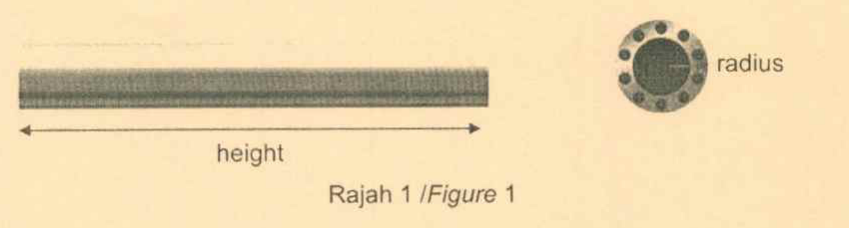
The engineering discipline of piping design studies the efficient transport of fluid. You are required to design a stable pipe that can hold 200 litres of fluid at a time. Assuming that it is a closed ended pipe at both ends, determine the dimensions (radius and height in cm) of the pipe that will minimize the amount of material used to construct the pipe with justification.

Solution

Let the pipe be a right circular cylinder of radius $r$ cm and height (length) $h$ cm.

Step 1 — Write down the constraint. The pipe must hold 200 litres of fluid, and $1 \ \text{litre} = 1000 \ \text{cm}^3$, so

$$V = \pi r^{2} h = 200 \times 1000 = 200\,000 \ \text{cm}^3 \quad\Longrightarrow\quad h = \frac{200\,000}{\pi r^{2}}.$$

Step 2 — Write the quantity to be minimized. "Amount of material" is the surface area of the metal sheet, and the pipe is closed at both ends, so it has two circular end caps plus the curved wall:

$$S = 2\pi r^{2} + 2\pi r h.$$

Substitute $h$ from the constraint to get a function of the single variable $r$:

$$S(r) = 2\pi r^{2} + 2\pi r \cdot \frac{200\,000}{\pi r^{2}} = 2\pi r^{2} + \frac{400\,000}{r}.$$

Step 3 — Minimize. Differentiate with respect to $r$ and set the derivative to zero:

$$\frac{dS}{dr} = 4\pi r - \frac{400\,000}{r^{2}} = 0 \quad\Longrightarrow\quad 4\pi r = \frac{400\,000}{r^{2}} \quad\Longrightarrow\quad r^{3} = \frac{100\,000}{\pi}.$$

Hence

$$r = \left(\frac{100\,000}{\pi}\right)^{1/3} \approx 31.69 \ \text{cm}.$$

Step 4 — Justify that this is a minimum. The second derivative is

$$\frac{d^{2}S}{dr^{2}} = 4\pi + \frac{800\,000}{r^{3}} > 0 \quad \text{for all } r > 0,$$

so $S$ is convex on $r > 0$ and the stationary point found is the global minimum (the function tends to $+\infty$ as $r \to 0^{+}$ and as $r \to \infty$, so there is no boundary minimum).

Step 5 — Recover $h$.

$$h = \frac{200\,000}{\pi r^{2}} = \frac{200\,000}{\pi \left(100\,000/\pi\right)^{2/3}} = 2\left(\frac{100\,000}{\pi}\right)^{1/3} = 2r \approx 63.38 \ \text{cm}.$$

The minimum material is

$$S_{\min} = 2\pi r^{2} + \frac{400\,000}{r} \approx 2\pi(31.69)^{2} + \frac{400\,000}{31.69} \approx 6310 + 12\,622 \approx 18\,932 \ \text{cm}^{2}.$$

So the optimum closed pipe is one whose height equals its diameter, $h = 2r$.

Answer: $r = \left(\dfrac{100\,000}{\pi}\right)^{1/3} \approx 31.7$ cm and $h = 2r \approx 63.4$ cm (minimum material $S_{\min} \approx 1.89 \times 10^{4}$ cm$^{2}$).

---

Question 1(b) (3 marks)

Question

The torsional rigidity of a length of a cable is calculated using the formula $N = \dfrac{8\pi E I}{t^{2} r^{4}}$. If $I$ is decreased by 2%, $r$ is increased by 1.5%, $t$ is increased by 1.5%. Can the cable still be used if the allowable limit for reduction in the torsional rigidity of a cable is 15%?

Solution

Method — small-change (logarithmic differentiation) error analysis. Take natural logarithms of the formula to turn the products and powers into a sum:

$$\ln N = \ln(8\pi E) + \ln I - 2\ln t - 4\ln r .$$

Differentiating gives the fractional (percentage) change relation

$$\frac{\delta N}{N} = \frac{\delta I}{I} - 2\,\frac{\delta t}{t} - 4\,\frac{\delta r}{r}.$$

Now insert the stated small changes:

Quantity	Change	Fractional change
$I$	decreased by 2%	$\delta I / I = -0.02$
$r$	increased by 1.5%	$\delta r / r = +0.015$
$t$	increased by 1.5%	$\delta t / t = +0.015$

$$\frac{\delta N}{N} = -0.02 - 2(0.015) - 4(0.015) = -0.02 - 0.03 - 0.06 = -0.11 .$$

So the torsional rigidity falls by 11%, i.e. $N$ becomes $0.89N$.

The allowable limit for the reduction is 15%, and

$$11\% < 15\%,$$

so the loss of torsional rigidity is within the permitted limit and the cable may still be used.

Answer: $\dfrac{\delta N}{N} = -11\%$, a reduction of 11% which is smaller than the allowable 15%, so yes — the cable can still be used.

---

Question 1(c) (7 marks)

Question

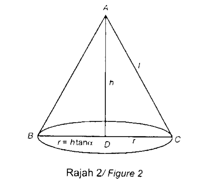
A conical-shaped exhaust product has the height $h$ and the semi-vertical angle $\alpha$ as shown in Figure 2. The total area $A$, including the base is calculated. If during manufacturing of the product, $h$ and $\alpha$ are in error by small quantities $\delta h$ and $\delta \alpha$ respectively, find the corresponding error in the area. Show that if $\alpha = \pi/6$, an error of 1% in $h$ will approximately compensated by an error of $-0.33^{\circ}$ in $\alpha$. [Hint: area of curved surface $= \pi r l$, where $l$ is the curved length]

Solution

Step 1 — Express the geometry through $h$ and $\alpha$. From the right-angled triangle in Figure 2 (apex $A$, centre of base $D$, rim $C$):

$$r = h\tan\alpha, \qquad l = \frac{h}{\cos\alpha} = h\sec\alpha .$$

Step 2 — Write the total area (curved surface + base).

$$A = \pi r l + \pi r^{2} = \pi (h\tan\alpha)(h\sec\alpha) + \pi (h\tan\alpha)^{2},$$$$A(h,\alpha) = \pi h^{2}\tan\alpha\,\sec\alpha + \pi h^{2}\tan^{2}\alpha = \pi h^{2}\tan\alpha\,(\sec\alpha + \tan\alpha).$$

Step 3 — Apply the total differential (small-error) formula.

$$\delta A \approx \frac{\partial A}{\partial h}\,\delta h + \frac{\partial A}{\partial \alpha}\,\delta\alpha .$$

Differentiate with respect to $h$ (treating $\alpha$ as constant):

$$\frac{\partial A}{\partial h} = 2\pi h\tan\alpha(\sec\alpha + \tan\alpha) = \frac{2A}{h}.$$

Differentiate with respect to $\alpha$ (treating $h$ as constant), using $\frac{d}{d\alpha}(\tan\alpha\sec\alpha) = \sec^{3}\alpha + \sec\alpha\tan^{2}\alpha$ and $\frac{d}{d\alpha}(\tan^{2}\alpha) = 2\tan\alpha\sec^{2}\alpha$:

$$\frac{\partial A}{\partial \alpha} = \pi h^{2}\left(\sec^{3}\alpha + \sec\alpha\tan^{2}\alpha + 2\tan\alpha\sec^{2}\alpha\right) = \frac{\pi h^{2}(1 + \sin\alpha)^{2}}{\cos^{3}\alpha}.$$

Therefore the error in the area is

$$\boxed{\ \delta A \approx 2\pi h\tan\alpha(\sec\alpha + \tan\alpha)\,\delta h + \frac{\pi h^{2}(1+\sin\alpha)^{2}}{\cos^{3}\alpha}\,\delta\alpha\ }$$

Step 4 — Specialize to $\alpha = \pi/6$. Here

$$\tan\frac{\pi}{6} = \frac{1}{\sqrt{3}}, \qquad \sec\frac{\pi}{6} = \frac{2}{\sqrt{3}}, \qquad \cos\frac{\pi}{6} = \frac{\sqrt{3}}{2}, \qquad \sin\frac{\pi}{6} = \frac{1}{2}.$$$$\tan\alpha(\sec\alpha + \tan\alpha) = \frac{1}{\sqrt{3}}\left(\frac{2}{\sqrt{3}} + \frac{1}{\sqrt{3}}\right) = \frac{1}{\sqrt{3}}\cdot\frac{3}{\sqrt{3}} = 1 \quad\Longrightarrow\quad A = \pi h^{2},$$$$\frac{\partial A}{\partial h}\Big|_{\alpha = \pi/6} = 2\pi h(1) = 2\pi h,$$$$\frac{\partial A}{\partial \alpha}\Big|_{\alpha = \pi/6} = \frac{\pi h^{2}\left(1 + \tfrac{1}{2}\right)^{2}}{\left(\tfrac{\sqrt{3}}{2}\right)^{3}} = \frac{\pi h^{2}\left(\tfrac{9}{4}\right)}{\tfrac{3\sqrt{3}}{8}} = \frac{9\pi h^{2}}{4}\cdot\frac{8}{3\sqrt{3}} = 2\sqrt{3}\,\pi h^{2}.$$

Step 5 — Compensation condition. A 1% error in $h$ means $\delta h = 0.01h$, so

$$\delta A = 2\pi h(0.01h) + 2\sqrt{3}\pi h^{2}\,\delta\alpha = 0.02\pi h^{2} + 2\sqrt{3}\pi h^{2}\,\delta\alpha .$$

For this to be approximately compensated we require $\delta A = 0$:

$$0.02\pi h^{2} + 2\sqrt{3}\pi h^{2}\,\delta\alpha = 0 \quad\Longrightarrow\quad \delta\alpha = -\frac{0.02}{2\sqrt{3}} = -\frac{0.01}{\sqrt{3}} \ \text{rad}.$$

Convert to degrees:

$$\delta\alpha = -\frac{0.01}{\sqrt{3}} \times \frac{180}{\pi} \approx -0.005773 \times 57.296 \approx -0.3308^{\circ} \approx -0.33^{\circ}.$$

This is exactly the stated result: at $\alpha = \pi/6$ a $+1\%$ error in the height is compensated (to first order) by an error of about $-0.33^{\circ}$ in the semi-vertical angle.

Answer: $\delta A \approx \dfrac{2A}{h}\,\delta h + 2\sqrt{3}\,\pi h^{2}\,\delta\alpha$ at $\alpha = \pi/6$, and the compensating angular error is $\delta\alpha = -\dfrac{0.01}{\sqrt{3}}$ rad $\approx -0.33^{\circ}$.

---

Question 2

Question 2(a) (7 marks)

Question

Given that matrix $A = \begin{pmatrix} 2 & 0 & 0 \\ 0 & 4 & 5 \\ 0 & 4 & 3 \end{pmatrix}$ can be diagonalized. Find the matrix that will diagonalize matrix $A$ if the diagonal matrix is $\begin{pmatrix} -1 & 0 & 0 \\ 0 & 2 & 0 \\ 0 & 0 & 8 \end{pmatrix}$.

Solution

Method. The matrix $P$ that diagonalizes $A$ has the eigenvectors of $A$ as its columns, ordered to match the given diagonal matrix $D = \operatorname{diag}(-1,\,2,\,8)$; then $P^{-1}AP = D$, i.e. $A = PDP^{-1}$.

Step 1 — Confirm the eigenvalues. Expand the characteristic determinant along the first row and factorise:

$$\det(A - \lambda I) = (2-\lambda)\left[(4-\lambda)(3-\lambda) - 20\right] = (2-\lambda)(\lambda^{2} - 7\lambda - 8) = (2-\lambda)(\lambda - 8)(\lambda + 1).$$

So $\lambda = 2,\ 8,\ -1$, which agrees with the given $D$.

Step 2 — Eigenvector for $\lambda = -1$ (first column of $P$). Solve $(A + I)\mathbf{x} = \mathbf{0}$:

$$\begin{pmatrix} 3 & 0 & 0 \\ 0 & 5 & 5 \\ 0 & 4 & 4 \end{pmatrix} \begin{pmatrix} x_{1} \\ x_{2} \\ x_{3} \end{pmatrix} = \mathbf{0} \quad\Longrightarrow\quad x_{1} = 0,\quad x_{2} + x_{3} = 0 .$$

Choose $x_{2} = 1$, $x_{3} = -1$:

$$\mathbf{v}_{1} = \begin{pmatrix} 0 \\ 1 \\ -1 \end{pmatrix}.$$

Step 3 — Eigenvector for $\lambda = 2$ (second column of $P$). Solve $(A - 2I)\mathbf{x} = \mathbf{0}$:

$$\begin{pmatrix} 0 & 0 & 0 \\ 0 & 2 & 5 \\ 0 & 4 & 1 \end{pmatrix} \begin{pmatrix} x_{1} \\ x_{2} \\ x_{3} \end{pmatrix} = \mathbf{0} \quad\Longrightarrow\quad 2x_{2} + 5x_{3} = 0,\quad 4x_{2} + x_{3} = 0 .$$

The last two equations force $x_{2} = x_{3} = 0$, while $x_{1}$ is free. Choose $x_{1} = 1$:

$$\mathbf{v}_{2} = \begin{pmatrix} 1 \\ 0 \\ 0 \end{pmatrix}.$$

Step 4 — Eigenvector for $\lambda = 8$ (third column of $P$). Solve $(A - 8I)\mathbf{x} = \mathbf{0}$:

$$\begin{pmatrix} -6 & 0 & 0 \\ 0 & -4 & 5 \\ 0 & 4 & -5 \end{pmatrix} \begin{pmatrix} x_{1} \\ x_{2} \\ x_{3} \end{pmatrix} = \mathbf{0} \quad\Longrightarrow\quad x_{1} = 0,\quad -4x_{2} + 5x_{3} = 0 .$$

Choose $x_{2} = 5$, $x_{3} = 4$:

$$\mathbf{v}_{3} = \begin{pmatrix} 0 \\ 5 \\ 4 \end{pmatrix}.$$

Step 5 — Assemble $P$ and verify. Taking the eigenvectors in the order $-1,\,2,\,8$ to match $D$:

$$P = \begin{pmatrix} 0 & 1 & 0 \\ 1 & 0 & 5 \\ -1 & 0 & 4 \end{pmatrix}.$$

Check each column: $A\mathbf{v}_{1} = -\mathbf{v}_{1}$, $A\mathbf{v}_{2} = 2\mathbf{v}_{2}$, $A\mathbf{v}_{3} = (0,\,40,\,32)^{T} = 8\mathbf{v}_{3}$. ✓

The inverse (from $\det P = -9$ and the adjoint) is

$$P^{-1} = \begin{pmatrix} 0 & \tfrac{4}{9} & -\tfrac{5}{9} \\[2pt] 1 & 0 & 0 \\[2pt] 0 & \tfrac{1}{9} & \tfrac{1}{9} \end{pmatrix},$$

and indeed

$$PDP^{-1} = \begin{pmatrix} 0 & 1 & 0 \\ 1 & 0 & 5 \\ -1 & 0 & 4 \end{pmatrix} \begin{pmatrix} -1 & 0 & 0 \\ 0 & 2 & 0 \\ 0 & 0 & 8 \end{pmatrix} \begin{pmatrix} 0 & \tfrac{4}{9} & -\tfrac{5}{9} \\ 1 & 0 & 0 \\ 0 & \tfrac{1}{9} & \tfrac{1}{9} \end{pmatrix} = \begin{pmatrix} 2 & 0 & 0 \\ 0 & 4 & 5 \\ 0 & 4 & 3 \end{pmatrix} = A. \ \checkmark$$

Answer: $P = \begin{pmatrix} 0 & 1 & 0 \\ 1 & 0 & 5 \\ -1 & 0 & 4 \end{pmatrix}$ diagonalizes $A$, with $P^{-1} = \begin{pmatrix} 0 & 4/9 & -5/9 \\ 1 & 0 & 0 \\ 0 & 1/9 & 1/9 \end{pmatrix}$ and $A = PDP^{-1}$ where $D = \operatorname{diag}(-1,\,2,\,8)$.

---

Question 2(b) (8 marks)

Question

A software developer company would like to invest in three new projects, namely projects A, B and C, which are expected to give 5%, 10% and 10% rates of return respectively. However, based on market preference, the company also decides that the amount invested for project B has to be twice the amount invested for project C. If the total investment amount and the total return for all three projects are 27500 and 2500 respectively, determine the amount invested for each project using the Cramer's method.

Solution

Step 1 — Set up the system of linear equations. Let $x$, $y$ and $z$ be the amounts (in the same currency units) invested in projects A, B and C.

Total investment:

$$x + y + z = 27\,500.$$

Total return (5% of $x$ plus 10% of $y$ plus 10% of $z$ equals 2500):

$$0.05x + 0.10y + 0.10z = 2500 .$$

Market-preference condition (B is twice C):

$$y = 2z \quad\Longrightarrow\quad y - 2z = 0 .$$

To keep integer entries, multiply the return equation by 100:

$$5x + 10y + 10z = 250\,000 .$$

In matrix form $M\mathbf{u} = \mathbf{b}$ with $\mathbf{u} = (x,\,y,\,z)^{T}$:

$$\begin{pmatrix} 1 & 1 & 1 \\ 5 & 10 & 10 \\ 0 & 1 & -2 \end{pmatrix} \begin{pmatrix} x \\ y \\ z \end{pmatrix} = \begin{pmatrix} 27\,500 \\ 250\,000 \\ 0 \end{pmatrix}.$$

Step 2 — Determinant of the coefficient matrix (Cramer's denominator).

$$\begin{aligned} \det M &= \begin{vmatrix} 1 & 1 & 1 \\ 5 & 10 & 10 \\ 0 & 1 & -2 \end{vmatrix} = 1\bigl[10(-2) - 10(1)\bigr] - 1\bigl[5(-2) - 10(0)\bigr] + 1\bigl[5(1) - 10(0)\bigr]\\ &= 1(-30) - 1(-10) + 1(5) = -30 + 10 + 5 = -15 \ne 0 . \end{aligned}$$

Since $\det M \ne 0$ the system has a unique solution and Cramer's rule applies.

Step 3 — Solve for $x$ (replace column 1 by $\mathbf{b}$):

$$\det M_{x} = \begin{vmatrix} 27\,500 & 1 & 1 \\ 250\,000 & 10 & 10 \\ 0 & 1 & -2 \end{vmatrix} = 27\,500(-30) - 1(-500\,000) + 1(250\,000) = -825\,000 + 500\,000 + 250\,000 = -75\,000,$$$$x = \frac{\det M_{x}}{\det M} = \frac{-75\,000}{-15} = 5000 .$$

Step 4 — Solve for $y$ (replace column 2 by $\mathbf{b}$). Expanding along the third row (only the entry $-2$ survives):

$$\det M_{y} = \begin{vmatrix} 1 & 27\,500 & 1 \\ 5 & 250\,000 & 10 \\ 0 & 0 & -2 \end{vmatrix} = (-2)\,(+1)\begin{vmatrix} 1 & 27\,500 \\ 5 & 250\,000 \end{vmatrix} = -2\,(250\,000 - 137\,500) = -225\,000,$$$$y = \frac{\det M_{y}}{\det M} = \frac{-225\,000}{-15} = 15\,000 .$$

Step 5 — Solve for $z$ (replace column 3 by $\mathbf{b}$):

$$\det M_{z} = \begin{vmatrix} 1 & 1 & 27\,500 \\ 5 & 10 & 250\,000 \\ 0 & 1 & 0 \end{vmatrix} = (1)(-1)^{3+2}\begin{vmatrix} 1 & 27\,500 \\ 5 & 250\,000 \end{vmatrix} = -(250\,000 - 137\,500) = -112\,500,$$$$z = \frac{\det M_{z}}{\det M} = \frac{-112\,500}{-15} = 7500 .$$

Step 6 — Check. $5000 + 15\,000 + 7500 = 27\,500$ ✓ and $0.05(5000) + 0.10(15\,000) + 0.10(7500) = 250 + 1500 + 750 = 2500$ ✓, with $y = 15\,000 = 2(7500) = 2z$ ✓.

Answer: Project A: $5000$, Project B: $15\,000$, Project C: $7500$ (so $x = 5000$, $y = 15\,000$, $z = 7500$).

---

Question 3

Question 3(i) (5 marks)

Question

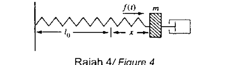
A spring of original length $l_{0}$ has a mass $m$ attached to it and a dashpot damping the motion. It is subject to a force $f(t)$ forcing the motion as shown in Figure 4.

The input to this system is the forcing function, $f(t)$ and the output is the displacement of the spring from its original length, $x(t)$. The system is satisfying the equation 1:

$$m\frac{d^{2}x}{dt^{2}} + r\frac{dx}{dt} + kx = f(t) \tag{1}$$

(i) Find all the possible complementary solutions for the displacement of the spring after time $t$. Let $\lambda = \text{root}$ in the calculation.

Solution

Method. The complementary solution $x_{c}(t)$ is the general solution of the homogeneous equation obtained by putting $f(t) = 0$. Try the exponential trial solution $x = e^{\lambda t}$, which converts the ODE into the auxiliary (characteristic) equation

$$m\lambda^{2} + r\lambda + k = 0 \quad\Longrightarrow\quad \lambda = \frac{-r \pm \sqrt{r^{2} - 4mk}}{2m}.$$

The form of $x_{c}$ is decided by the sign of the discriminant $\Delta = r^{2} - 4mk$.

Case 1 — Two distinct real roots: $r^{2} > 4mk$ (overdamped).

$$\lambda_{1} = \frac{-r + \sqrt{r^{2} - 4mk}}{2m}, \qquad \lambda_{2} = \frac{-r - \sqrt{r^{2} - 4mk}}{2m},$$$$x_{c}(t) = C_{1}e^{\lambda_{1} t} + C_{2}e^{\lambda_{2} t}.$$

Case 2 — One repeated real root: $r^{2} = 4mk$ (critically damped).

$$\lambda_{1} = \lambda_{2} = \lambda = -\frac{r}{2m},$$

and the second independent solution is $t e^{\lambda t}$, so

$$x_{c}(t) = (C_{1} + C_{2}t)\,e^{-rt/(2m)}.$$

Case 3 — Complex conjugate roots: $r^{2} < 4mk$ (underdamped). Writing

$$\lambda = -\frac{r}{2m} \pm i\omega, \qquad \omega = \frac{\sqrt{4mk - r^{2}}}{2m} \ (> 0),$$

Euler's formula gives the real form

$$x_{c}(t) = e^{-rt/(2m)}\left(C_{1}\cos\omega t + C_{2}\sin\omega t\right).$$

In every case $C_{1}$ and $C_{2}$ are arbitrary constants fixed by the initial displacement $x(0)$ and initial velocity $x'(0)$.

Answer: With $\lambda = \dfrac{-r \pm \sqrt{r^{2} - 4mk}}{2m}$: if $r^{2} > 4mk$, $x_{c} = C_{1}e^{\lambda_{1}t} + C_{2}e^{\lambda_{2}t}$; if $r^{2} = 4mk$, $x_{c} = (C_{1} + C_{2}t)e^{-rt/(2m)}$; if $r^{2} < 4mk$, $x_{c} = e^{-rt/(2m)}\left(C_{1}\cos\omega t + C_{2}\sin\omega t\right)$ with $\omega = \dfrac{\sqrt{4mk - r^{2}}}{2m}$.

---

Question 3(ii) (2 marks)

Question

Based on the result in part b(i), design the value of $r$ for repeated root case so that displacement can be minimized, if $m$ and $k$ are given as 2 and 2048 respectively. Hence, find the complementary solution. Note: $r > 0$.

Solution

Step 1 — Impose the repeated-root condition. A repeated root occurs when the discriminant vanishes:

$$r^{2} - 4mk = 0 \quad\Longrightarrow\quad r = \sqrt{4mk} = 2\sqrt{mk}.$$

With $m = 2$ and $k = 2048$:

$$r = 2\sqrt{(2)(2048)} = 2\sqrt{4096} = 2(64) = 128 .$$

(We take $r = +128$ since $r > 0$.)

Step 2 — Why this design minimizes the displacement. This is the critically damped case. Because the discriminant is zero there is no oscillation and no overshoot: the displacement decays to zero monotonically, and of all non-oscillatory choices it decays fastest. If $r < 2\sqrt{mk}$ (underdamped) the mass oscillates about equilibrium, and if $r > 2\sqrt{mk}$ (overdamped) the extra damping slows the return. Hence the repeated-root (critical) value minimizes the displacement over time.

Step 3 — Complementary solution. The repeated root is

$$\lambda = -\frac{r}{2m} = -\frac{128}{2(2)} = -32 .$$

Therefore

$$x_{c}(t) = (C_{1} + C_{2}t)e^{-32t}.$$

Answer: $r = 2\sqrt{mk} = 128$, giving the repeated root $\lambda = -32$ and $x_{c}(t) = (C_{1} + C_{2}t)e^{-32t}$.

---

Question 3(iii) (8 marks)

Question

Hence, solve the total displacement solution for the designed parameters ($m$, $r$, and $k$) in part b(ii) if $f(t) = te^{t}$. Then, estimate $x(t)$ when $t = 10$.

Solution

Step 1 — Write the equation for the designed parameters. With $m = 2$, $r = 128$ and $k = 2048$, equation (1) becomes

$$2\frac{d^{2}x}{dt^{2}} + 128\frac{dx}{dt} + 2048x = te^{t}.$$

The total solution is $x(t) = x_{c}(t) + x_{p}(t)$, where $x_{c}(t) = (C_{1} + C_{2}t)e^{-32t}$ from part (ii).

Step 2 — Choose the trial particular integral. The right-hand side is $te^{t}$, and $e^{t}$ is not a root of the auxiliary equation ($\lambda = -32$), so use the undetermined-coefficients form

$$x_{p}(t) = (at + b)e^{t}.$$

Then

$$x_{p}' = (at + b + a)e^{t}, \qquad x_{p}'' = (at + b + 2a)e^{t}.$$

Step 3 — Substitute and match coefficients.

$$\begin{aligned} 2x_{p}'' + 128x_{p}' + 2048x_{p} &= \bigl[2(at + b + 2a) + 128(at + b + a) + 2048(at + b)\bigr]e^{t}\\ &= \bigl[2178\,at + (2178b + 132a)\bigr]e^{t} \stackrel{!}{=} te^{t}. \end{aligned}$$

Comparing coefficients of $t$ and of the constant term:

$$2178a = 1 \quad\Longrightarrow\quad a = \frac{1}{2178},$$$$2178b + 132a = 0 \quad\Longrightarrow\quad b = -\frac{132}{2178}a = -\frac{132}{2178^{2}} = -\frac{1}{35937}.$$

Hence

$$x_{p}(t) = \left(\frac{t}{2178} - \frac{1}{35937}\right)e^{t}.$$

Step 4 — Write the general (total) solution.

$$x(t) = (C_{1} + C_{2}t)e^{-32t} + \left(\frac{t}{2178} - \frac{1}{35937}\right)e^{t}.$$

Step 5 — Estimate $x(10)$. Put $t = 10$:

$$x(10) = (C_{1} + 10C_{2})e^{-320} + \left(\frac{10}{2178} - \frac{1}{35937}\right)e^{10}.$$

The homogeneous (transient) term contains $e^{-320} \approx 1.06 \times 10^{-139}$, which is utterly negligible, so it dies away long before $t = 10$:

$$x(10) \approx \left(0.0045914 - 0.0000278\right)\left(22\,026.47\right) \approx (0.0045635)(22\,026.47) \approx 100.5 .$$

Answer: $x(t) = (C_{1} + C_{2}t)e^{-32t} + \left(\dfrac{t}{2178} - \dfrac{1}{35937}\right)e^{t}$, and $x(10) \approx 100.5$ (the transient term is $\sim 10^{-139}$, i.e. zero to any practical accuracy).

Printing inconsistency in the paper

Parts (i)–(iii) of Question 3 are labelled with Roman numerals, but the wording of parts (ii) and (iii) refers to "part b(i)" and "part b(ii)". There is no part (b) in Question 3; these references are read as parts (i) and (ii) of Question 3.

---

Question 4

Question 4(a) (12 marks)

Question

Hydraulic impact hammer (Figure 5) characteristics can be defined by the following second order differential equation (equation 2). Based on the initial values, find the particular solution using power series and present the solution with at least 5 partial summation terms.

Figure 5

Figure 5 is a labelled cross-section of the hydraulic impact hammer showing the coupler, housing, back head, valve, accumulator, upper piston, main body and chisel. It is illustrative only — equation (2) and the initial conditions (3) below contain everything needed to solve the problem.

$$y'' - 6xy' + x^{2}y = 0 \tag{2}$$ $$y(0) = 2, \qquad y'(0) = 1 \tag{3}$$

Solution

Method — power series solution about the ordinary point $x = 0$.

Step 1 — Assume a power series solution.

$$y = \sum_{n=0}^{\infty} a_{n}x^{n}, \qquad y' = \sum_{n=1}^{\infty} n a_{n}x^{n-1}, \qquad y'' = \sum_{n=2}^{\infty} n(n-1)a_{n}x^{n-2}.$$

Step 2 — Substitute into equation (2).

$$\underbrace{\sum_{n=2}^{\infty} n(n-1)a_{n}x^{n-2}}_{(I)} - 6\underbrace{\sum_{n=1}^{\infty} n a_{n}x^{n}}_{(II)} + \underbrace{\sum_{n=0}^{\infty} a_{n}x^{n+2}}_{(III)} = 0 .$$

Re-index so that every series carries the same power $x^{m}$:

• $(I)$: put $m = n - 2$, so $n = m + 2$: $\displaystyle\sum_{m=0}^{\infty}(m+2)(m+1)a_{m+2}x^{m}$;
• $(II)$: already $\displaystyle\sum_{m=1}^{\infty} m a_{m}x^{m}$;
• $(III)$: put $m = n + 2$, so $n = m - 2$: $\displaystyle\sum_{m=2}^{\infty} a_{m-2}x^{m}$.

Step 3 — Recurrence relation. Collecting the coefficient of $x^{m}$ gives

$$(m+2)(m+1)a_{m+2} - 6m\,a_{m} + a_{m-2} = 0 \qquad (m \ge 0,\ \ a_{-2} = 0),$$$$\boxed{\ a_{m+2} = \frac{6m\,a_{m} - a_{m-2}}{(m+2)(m+1)}\ }$$

where the term $a_{m-2}$ is present only for $m \ge 2$.

Step 4 — Initial values. From $y(0) = 2$ and $y'(0) = 1$:

$$a_{0} = 2, \qquad a_{1} = 1 .$$

Step 5 — Generate the coefficients from the recurrence.

$m$	Recurrence	Coefficient
0	$a_{2} = \dfrac{0 - 0}{2\cdot 1}$	$a_{2} = 0$
1	$a_{3} = \dfrac{6(1)(1) - 0}{3\cdot 2} = \dfrac{6}{6}$	$a_{3} = 1$
2	$a_{4} = \dfrac{12(0) - 2}{4\cdot 3} = \dfrac{-2}{12}$	$a_{4} = -\dfrac{1}{6}$
3	$a_{5} = \dfrac{18(1) - 1}{5\cdot 4} = \dfrac{17}{20}$	$a_{5} = \dfrac{17}{20}$
4	$a_{6} = \dfrac{24\left(-\tfrac{1}{6}\right) - 0}{6\cdot 5} = \dfrac{-4}{30}$	$a_{6} = -\dfrac{2}{15}$
5	$a_{7} = \dfrac{30\left(\tfrac{17}{20}\right) - 1}{7\cdot 6} = \dfrac{24.5}{42}$	$a_{7} = \dfrac{7}{12}$
6	$a_{8} = \dfrac{36\left(-\tfrac{2}{15}\right) - \left(-\tfrac{1}{6}\right)}{8\cdot 7} = \dfrac{-\tfrac{139}{30}}{56}$	$a_{8} = -\dfrac{139}{1680}$

Step 6 — Particular solution. Substituting back,

$$y(x) = 2 + x + 0\cdot x^{2} + x^{3} - \frac{1}{6}x^{4} + \frac{17}{20}x^{5} - \frac{2}{15}x^{6} + \frac{7}{12}x^{7} - \frac{139}{1680}x^{8} + \cdots$$

i.e. nine partial-summation terms (eight of them non-zero — well over the five required). As a check, the recurrence at $m = 6$ reads $56a_{8} - 36a_{6} + a_{4} = -\frac{139}{30} + \frac{24}{5} - \frac{1}{6} = 0$ ✓, and a numerical integration of the ODE with $y(0)=2$, $y'(0)=1$ reproduces the series to 7 decimal places at small $x$.

Answer:

$$y(x) = 2 + x + x^{3} - \frac{1}{6}x^{4} + \frac{17}{20}x^{5} - \frac{2}{15}x^{6} + \frac{7}{12}x^{7} - \frac{139}{1680}x^{8} + \cdots$$

(from $a_{m+2} = \dfrac{6m a_{m} - a_{m-2}}{(m+2)(m+1)}$, $a_{0} = 2$, $a_{1} = 1$).

---

Question 4(b) (3 marks)

Question

Determine the singular point type of the given differential equations and whether they can be solved by power series or not.

Differential Equation	Singular point type	Power series (Yes or No)
$8x^{2}y'' + 10xy' + (x-1)y = 0$
$y'' + x^{4}y' + y = 0$
$2(x-1)^{2}y'' + x^{4}y' + y = 0$

Solution

Method. Write each equation in the standard form

$$y'' + p(x)y' + q(x)y = 0 .$$

A point $x_{0}$ is a singular point if $p$ or $q$ fails to be analytic there. It is a regular singular point when both $(x - x_{0})p(x)$ and $(x - x_{0})^{2}q(x)$ are analytic at $x_{0}$ (then the Frobenius/power-series method works); otherwise it is an irregular singular point (no power-series solution about $x_{0}$). If $p$ and $q$ are analytic at $x_{0}$, then $x_{0}$ is an ordinary point and an ordinary power series solution always exists.

(1) $8x^{2}y'' + 10xy' + (x-1)y = 0$. Dividing by $8x^{2}$:

$$y'' + \frac{10}{8x}y' + \frac{x-1}{8x^{2}}y = 0 \quad\Longrightarrow\quad p(x) = \frac{5}{4x}, \quad q(x) = \frac{x-1}{8x^{2}}.$$

$x = 0$ is the only singular point. Test it:

$$x\,p(x) = \frac{5}{4} \ \text{(analytic at } x=0), \qquad x^{2}q(x) = \frac{x-1}{8} \ \text{(analytic at } x=0).$$

Both are analytic, so $x = 0$ is a regular singular point and the equation can be solved by (Frobenius) power series — the indicial equation comes from $r(r-1) + \tfrac{5}{4}r - \tfrac{1}{8} = 0$.

(2) $y'' + x^{4}y' + y = 0$. Here $p(x) = x^{4}$ and $q(x) = 1$ are polynomials, hence analytic everywhere. There is no singular point (every point, in particular $x = 0$, is an ordinary point), so an ordinary power series solution $y = \sum a_{n}x^{n}$ exists for all $x$ — Yes.

(3) $2(x-1)^{2}y'' + x^{4}y' + y = 0$. Dividing by $2(x-1)^{2}$:

$$y'' + \frac{x^{4}}{2(x-1)^{2}}y' + \frac{1}{2(x-1)^{2}}y = 0 \quad\Longrightarrow\quad p(x) = \frac{x^{4}}{2(x-1)^{2}}, \quad q(x) = \frac{1}{2(x-1)^{2}}.$$

The only singular point is $x = 1$. Test it:

$$(x-1)p(x) = \frac{x^{4}}{2(x-1)} \ \text{is not analytic at } x = 1,$$

so the singularity is an irregular singular point and the equation cannot be solved by a power series about $x = 1$ — No.

The completed table:

Differential Equation	Singular point type	Power series (Yes or No)
$8x^{2}y'' + 10xy' + (x-1)y = 0$	Regular singular point at $x = 0$	Yes
$y'' + x^{4}y' + y = 0$	No singular point ($x=0$ ordinary)	Yes
$2(x-1)^{2}y'' + x^{4}y' + y = 0$	Irregular singular point at $x = 1$	No

Answer:

Differential Equation	Singular point type	Power series
$8x^{2}y'' + 10xy' + (x-1)y = 0$	Regular singular point ($x = 0$)	Yes
$y'' + x^{4}y' + y = 0$	No singular point — ordinary point ($x = 0$)	Yes
$2(x-1)^{2}y'' + x^{4}y' + y = 0$	Irregular singular point ($x = 1$)	No

About the third equation

$x = 0$ is an ordinary point of $2(x-1)^{2}y'' + x^{4}y' + y = 0$, so a power series about $x = 0$ does exist. The classification above is about the equation's singular point $x = 1$; because that singularity is irregular, no power-series (Frobenius) solution about $x = 1$ is possible.

---

Appendix 1

The paper supplies the following formula sheets (Appendix 1, page 7 of the original).

Table 1: Trigonometry Differentiation Formula

$$\frac{d}{dx}(\sin x) = \cos x, \qquad \frac{d}{dx}(\cos x) = -\sin x, \qquad \frac{d}{dx}(\tan x) = (\sec x)^{2},$$ $$\frac{d}{dx}(\sec x) = \sec x\cdot\tan x, \qquad \frac{d}{dx}(\csc x) = -\csc x\cdot\cot x, \qquad \frac{d}{dx}(\cot x) = -(\csc x)^{2}.$$

Table 2: Commons forms of 2nd order ODE and strategy to solve them

Forms	Strategy
Homogeneous linear differential equation with constant coefficients $a,\ b,\ c$: $a\dfrac{d^{2}y}{dx^{2}} + b\dfrac{dy}{dx} + cy = 0$	Let $y(x) = e^{mx}$ and use characteristic equation
Nonhomogeneous linear differential equation with constant coefficients $a,\ b,\ c$ in the form of $r(x) = e^{\alpha x}P_{n}(x)$: $a\dfrac{d^{2}y}{dx^{2}} + b\dfrac{dy}{dx} + cy = r(x)$	Method of undetermined coefficients
All types of nonhomogeneous linear differential equation: $\dfrac{d^{2}y}{dx^{2}} + p(x)\dfrac{dy}{dx} + q(x)y = r(x)$	Method of variation of parameters

Where the appendix is used above.

• Question 3(i) uses Table 2, row 1 — the characteristic equation $m\lambda^{2} + r\lambda + k = 0$ for the homogeneous equation.
• Question 3(iii) uses Table 2, row 2 — the method of undetermined coefficients for $r(t) = te^{t} = e^{1\cdot t}P_{1}(t)$ with $P_{1}(t) = t$.
• Question 1(c) uses the trigonometric derivatives of Table 1 to differentiate $\tan\alpha\sec\alpha$ and $\tan^{2}\alpha$: $\frac{d}{d\alpha}(\tan\alpha\sec\alpha) = \sec^{3}\alpha + \sec\alpha\tan^{2}\alpha$ and $\frac{d}{d\alpha}(\tan^{2}\alpha) = 2\tan\alpha\sec^{2}\alpha$.
• Question 4(b) uses Table 2, rows 1 and 3 to identify the applicable solution strategy at ordinary and singular points.

TAMAT / END — 7 printed pages.