Tutorial 6

Tutorial 6: Matrix Algebra for Non-Homogeneous Linear Algebraic System

Tutorial QuestionTutorial Solution

1. Solve the unknown $\boldsymbol{F}$ for the following equation:

   $$\begin{aligned} & \frac{1}{4}\left[\frac{220}{\operatorname{trace}(\boldsymbol{C})} \mathbf{A}^{\boldsymbol{T}} . \mathbf{B}-\mathbf{C}\right]=\frac{1}{3} \boldsymbol{E} \boldsymbol{F}-\frac{20}{\operatorname{determinant}(\mathbf{D})} \mathbf{D} \\ & \text { where } \mathbf{A}=\left[\begin{array}{ccc}1 & 0 & 2 \\3 & -1 & -3\end{array}\right], \mathbf{B}=\left[\begin{array}{ccc}4 & 6 & 8 \\-2 & 5 & 7\end{array}\right], \mathbf{C}=\left[\begin{array}{ccc}10 & 11 & 3 \\-10 & -27 & -25 \\70 & -29 & -27\end{array}\right] \\ & \mathbf{D}=\left[\begin{array}{ccc}1 & 2 & 0 \\-1 & 3 & 0 \\0 & 0 & 4\end{array}\right], \mathbf{E}=\left[\begin{array}{ccc}2 & -2 & 1 \\1 & 2 & 2 \\2 & 1 & -2\end{array}\right] \end{aligned}$$

   $\frac{1}{3} \boldsymbol{E}=$ orthogonal matrix if $\left(\frac{1}{3} \boldsymbol{E}\right)^{-1}=\left(\frac{1}{3} \boldsymbol{E}\right)^{T}$, verify if $\frac{1}{3} \boldsymbol{E}$ is an orthogonal matrix or not, hence use it for the calculation.

   Solution

   $$\begin{aligned} \boldsymbol{F}&=\left(\frac{1}{3} \boldsymbol{E}\right)^{-1}\left(\frac{1}{4}\left[\frac{220}{\operatorname{trace}(\boldsymbol{C})} \mathbf{A}^T . \mathbf{B}-\mathbf{C}\right]+\frac{20}{\operatorname{determinant}(\mathbf{D})} \mathbf{D}\right)\\ \boldsymbol{F}&=\left(\frac{1}{3} \boldsymbol{E}\right)^T\left(\frac{1}{4}\left[\frac{220}{\operatorname{trace}(\boldsymbol{C})} \mathbf{A}^T \text {. B }-\mathbf{C}\right]+\frac{20}{\operatorname{determinant}(\mathbf{D})} \mathbf{D}\right) \end{aligned}$$

   $\operatorname{trace}(\boldsymbol{C})=10-27-27=-44$

   $$\begin{aligned} \mathbf{A}^{\boldsymbol{T}}&=\left[\begin{array}{cc} 1 & 3 \\ 0 & -1 \\ 2 & -3 \end{array}\right]\\ \mathbf{A}^{\boldsymbol{T}} \cdot \mathbf{B}&=\left[\begin{array}{cc} 1 & 3 \\ 0 & -1 \\ 2 & -3 \end{array}\right]\left[\begin{array}{ccc} 4 & 6 & 8 \\ -2 & 5 & 7 \end{array}\right]=\left[\begin{array}{ccc} -2 & 21 & 29 \\ 2 & -5 & -7 \\ 14 & -3 & -5 \end{array}\right] \end{aligned}$$

   $$\begin{aligned} \frac{1}{4}\left[\frac{220}{\operatorname{trace}(\boldsymbol{C})} \mathbf{A}^T \cdot \mathbf{B}-\mathbf{C}\right]&=\frac{1}{4}\left[\frac{220}{-44}\left[\begin{array}{ccc} -2 & 21 & 29 \\ 2 & -5 & -7 \\ 14 & -3 & -5 \end{array}\right]-\left[\begin{array}{ccc} 10 & 11 & 3 \\ -10 & -27 & -25 \\ 70 & -29 & -27 \end{array}\right]\right]\\ &\begin{aligned} &=\frac{1}{4}\left[\left[\begin{array}{ccc} 10 & -105 & -145 \\ -10 & 25 & 35 \\ -70 & 15 & 25 \end{array}\right]-\left[\begin{array}{ccc} 10 & 11 & 3 \\ -10 & -27 & -25 \\ 70 & -29 & -27 \end{array}\right]\right. \\ &=\frac{1}{4}\left[\left[\begin{array}{ccc} 0 & -116 & -148 \\ 0 & 52 & 60 \\ -140 & 44 & 52 \end{array}\right]\right]=\left[\begin{array}{ccc} 0 & -29 & -37 \\ 0 & 13 & 15 \\ -35 & 11 & 13 \end{array}\right] \end{aligned} \end{aligned}$$

   $$\begin{aligned} \operatorname{determinant}(\mathbf{D})&=\left|\begin{array}{ccc} 1 & 2 & 0 \\ -1 & 3 & 0 \\ 0 & 0 & 4 \end{array}\right|=1(12)-2(-4)=20\\ \frac{20}{\text { determinant }(\mathbf{D})} \mathbf{D}&=\frac{20}{20}\left[\begin{array}{ccc} 1 & 2 & 0 \\ -1 & 3 & 0 \\ 0 & 0 & 4 \end{array}\right]=\left[\begin{array}{ccc} 1 & 2 & 0 \\ -1 & 3 & 0 \\ 0 & 0 & 4 \end{array}\right]\\ \end{aligned}$$

   $$\begin{aligned} \left(\frac{1}{4}\left[\frac{220}{\operatorname{trace}(\boldsymbol{C})} \mathbf{A}^{\boldsymbol{T}} \cdot \mathbf{B}-\mathbf{C}\right]+\frac{20}{\operatorname{determinant}(\mathbf{D})} \mathbf{D}\right) &=\left[\begin{array}{ccc} 0 & -29 & -37 \\ 0 & 13 & 15 \\ -35 & 11 & 13 \end{array}\right]+\left[\begin{array}{ccc} 1 & 2 & 0 \\ -1 & 3 & 0 \\ 0 & 0 & 4 \end{array}\right]\\ &=\left[\begin{array}{ccc} 1 & -27 & -37 \\ -1 & 16 & 15 \\ -35 & 11 & 17 \end{array}\right] \end{aligned}$$

   $$\left(\frac{1}{3} \boldsymbol{E}\right)^{-1}=\left[\begin{array}{ccc} 2 / 3 & -2 / 3 & 1 / 3 \\ 1 / 3 & 2 / 3 & 2 / 3 \\ 2 / 3 & 1 / 3 & -2 / 3 \end{array}\right]^{-1}=\frac{1}{\operatorname{det}\left(\frac{1}{3} \boldsymbol{E}\right)} \operatorname{adjoint}\left(\frac{1}{3} \boldsymbol{E}\right)$$

   $$\begin{aligned} \operatorname{cofactor}\left(\frac{1}{3}\boldsymbol{E}\right)=& \left[ \begin{array}{ccc} \left| \begin{array}{cc} 2/3 & 2/3 \\ 1/3 & -2/3 \end{array} \right| & -\left| \begin{array}{cc} 1/3 & 2/3 \\ 2/3 & -2/3 \end{array} \right| & \left| \begin{array}{cc} 1/3 & 2/3 \\ 2/3 & 1/3 \end{array} \right| \\ -2/3 & 1/3 & 1/3 \\ & & -2/3 \end{array} \right] \left| \begin{array}{cc} 2/3 & 1/3 \\ 2/3 & -2/3 \end{array} \right| \\ &- \left|\begin{array}{cc} 2 / 3 & -2 / 3 \\ 2 / 3 & 1 / 3 \end{array}\right|\left|\begin{array}{cc} -2 / 3 & 1 / 3 \\ 2 / 3 & 2 / 3 \end{array}\right|-\left|\begin{array}{cc} 2 / 3 & 1 / 3 \\ 1 / 3 & 2 / 3 \end{array}\right|\left|\begin{array}{cc} 2 / 3 & -2 / 3 \\ 1 / 3 & 2 / 3 \end{array}\right| \\ &=\left[\begin{array}{ccc} -2 / 3 & 2 / 3 & -1 / 3 \\ -1 / 3 & -2 / 3 & -2 / 3 \\ -2 / 3 & -1 / 3 & 2 / 3 \end{array}\right] \end{aligned}$$

   $$\text { adjoint }\left(\frac{1}{3} \boldsymbol{E}\right)=\left[\text { cofactor }\left(\frac{1}{3} \boldsymbol{E}\right)\right]^T=\left[\begin{array}{ccc} -2 / 3 & -1 / 3 & -2 / 3 \\ 2 / 3 & -2 / 3 & -1 / 3 \\ -1 / 3 & -2 / 3 & 2 / 3 \end{array}\right]$$

   $$\operatorname{det}\left(\frac{1}{3} \boldsymbol{E}\right)=\left|\begin{array}{ccc} 2 / 3 & -2 / 3 & 1 / 3 \\ 1 / 3 & 2 / 3 & 2 / 3 \\ 2 / 3 & 1 / 3 & -2 / 3 \end{array}\right|=-1$$

   $$\left(\frac{1}{3} \boldsymbol{E}\right)^{-1}=\frac{1}{-1}\left[\begin{array}{ccc} -2 / 3 & -1 / 3 & -2 / 3 \\ 2 / 3 & -2 / 3 & -1 / 3 \\ -1 / 3 & -2 / 3 & 2 / 3 \end{array}\right]=\left[\begin{array}{ccc} 2 / 3 & 1 / 3 & 2 / 3 \\ -2 / 3 & 2 / 3 & 1 / 3 \\ 1 / 3 & 2 / 3 & -2 / 3 \end{array}\right]$$

   $$\left(\frac{1}{3} \boldsymbol{E}\right)^T=\left[\begin{array}{ccc} 2 / 3 & -2 / 3 & 1 / 3 \\ 1 / 3 & 2 / 3 & 2 / 3 \\ 2 / 3 & 1 / 3 & -2 / 3 \end{array}\right]^T=\left[\begin{array}{ccc} 2 / 3 & 1 / 3 & 2 / 3 \\ -2 / 3 & 2 / 3 & 1 / 3 \\ 1 / 3 & 2 / 3 & -2 / 3 \end{array}\right]$$

   $\therefore$ It is verified that $\frac{1}{3} \boldsymbol{E}$ is an orthogonal matrix, where $\left(\frac{1}{3} \boldsymbol{E}\right)^{-1}=\left(\frac{1}{3} \boldsymbol{E}\right)^T$

   $$\begin{aligned} \boldsymbol{F} &=\left(\frac{1}{3} \boldsymbol{E}\right)^T\left(\frac{1}{4}\left[\frac{220}{\operatorname{trace}(\boldsymbol{C})} \mathbf{A}^T \cdot \mathbf{B}-\mathbf{C}\right]+\frac{20}{\operatorname{determinant}(\mathbf{D})} \mathbf{D}\right) \\ &=\left[\begin{array}{ccc} 2 / 3 & 1 / 3 & 2 / 3 \\ -2 / 3 & 2 / 3 & 1 / 3 \\ 1 / 3 & 2 / 3 & -2 / 3 \end{array}\right]\left[\begin{array}{ccc} 1 & -27 & -37 \\ -1 & 16 & 15 \\ -35 & 11 & 17 \end{array}\right] \\ &=\left[\begin{array}{ccc} -23 & -16 / 3 & -25 / 3 \\ -13 & 97 / 3 & 121 / 3 \\ 23 & -17 / 3 & -41 / 3 \end{array}\right] \end{aligned}$$

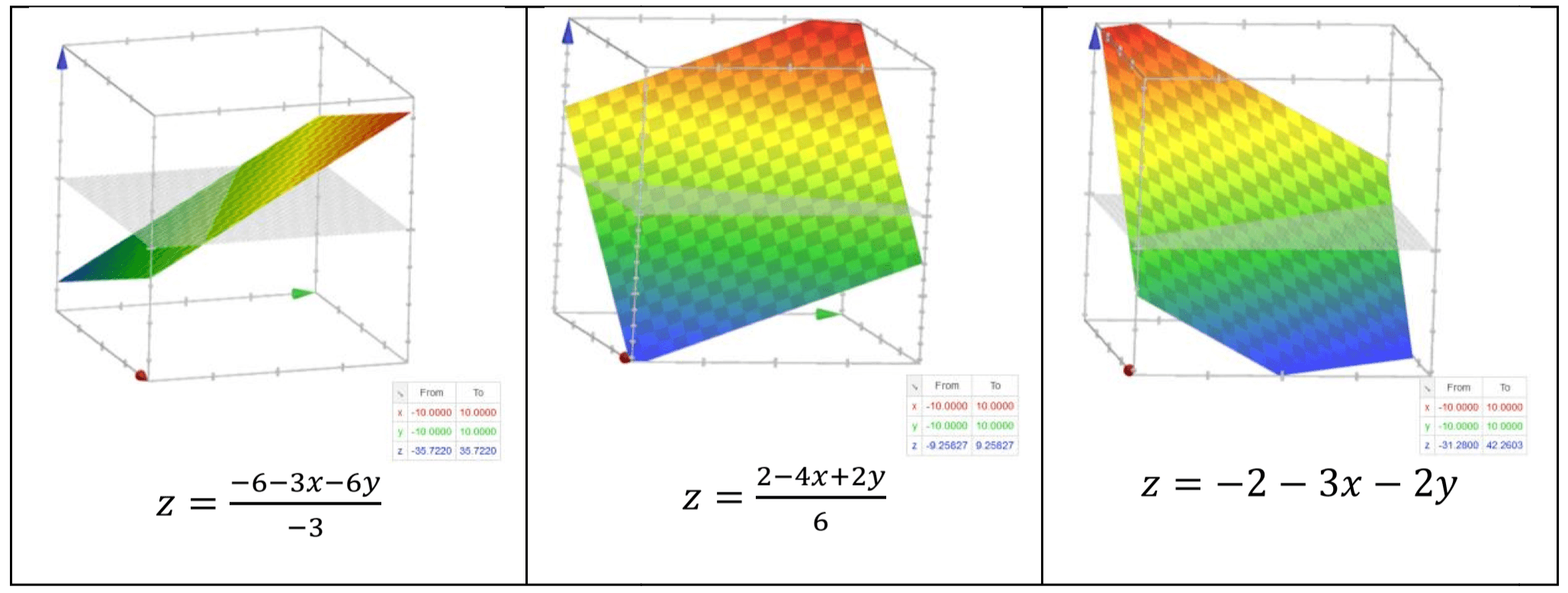
2. Choose the correct graph for each case, then comment on the condition of the coefficient matrix in terms of its determinant and the characteristic of the solution without solving it.

   Case 1	Case 2	Case 3
   $\begin{aligned} 3x_2+7x_1&=-5\\x_2-2x_1&=\frac{1}{2}\end{aligned}$	$\begin{aligned} x_2+2x_1&=4\\2x_2+3.999x_1&=7.999\end{aligned}$	$\begin{aligned} 5x_2+20x_1&=-1\\x_2+4x_1&=2\end{aligned}$

   

   Solution

   Case 1

   $$\begin{aligned} 3 x_2+7 x_1&=-5 \\ x_2-2 x_1&=\frac{1}{2} \\ \end{aligned}$$

   $$\begin{aligned} x_2&=-\left(\frac{7}{3}\right) x_1+\left(\frac{-5}{3}\right) \\ x_2&=2 x_1+(0.5) \end{aligned}$$

   Graph (c).

   There is one interception point. The coefficient matrix is well-conditioned where the determinant $\neq$ 0 (i.e. Huge slope difference).

   There is unique solution for a well-conditioned system.

   ---

   Case 2

   $$\begin{aligned} x_2+2 x_1&=4 \\ 2 x_2+3.999 x_1&=7.999 \end{aligned}$$

   $$\begin{aligned} x_2&=-2 x_1+(4) \\ x_2&=-\left(\frac{3.999}{2}\right) x_1+\left(\frac{7.999}{2}\right) \end{aligned}$$

   Graph (a).

   There are many interception points. The coefficient matrix is ill-conditioned where the determinant $\approx$ 0 (i.e. Close slope).

   There are many solutions for an ill-conditioned system and the solutions are sensitive to the noise.

   ---

   Case 3

   $$\begin{aligned} 5 x_2+20 x_1&=-1\\ x_2+4 x_1&=2 \end{aligned}$$

   $$\begin{aligned} x_2&=-4 x_1+\left(\frac{-1}{5}\right)\\ x_2&=-4 x_1+2 \end{aligned}$$

   Graph (b).

   There is no interception points. The coefficient matrix is singular where the determinant = 0 (i.e. Exact same slope).

   There is no solutions for the singular system which has no interception points.

3. Continue to solve Q2 by using Cramer's rule. Hence, verify the solution.

Solution

Case 1

$$\begin{aligned} 3 x_2+7 x_1&=-5\\ x_2-2 x_1&=\frac{1}{2} \end{aligned}$$

$$\begin{aligned} x_1&=\frac{\left|\begin{array}{cc} -5 & 7 \\ \frac{1}{2} & -2 \end{array}\right|}{\left|\begin{array}{cc} 3 & 7 \\ 1 & -2 \end{array}\right|} \\ &=\frac{6.5}{-13}=-0.5\\ x_2&=\frac{\left|\begin{array}{cc} 3 & -5 \\ 1 & \frac{1}{2} \end{array}\right|}{\left|\begin{array}{cc} 3 & 7 \\ 1 & -2 \end{array}\right|}\\ &=\frac{6.5}{-13}=-0.5\\ \end{aligned}$$

$$\left[\begin{array}{cc} 3 & 7 \\ 1 & -2 \end{array}\right]\left\{\begin{array}{c} -0.5 \\ -0.5 \end{array}\right\}\\ =\left\{\begin{array}{c} -5 \\ 0.5 \end{array}\right\}$$

(verified)

---

Case 2

$$\begin{aligned} x_2+2 x_1&=4\\ 2 x_2+3.999 x_1&=7.999\\ \end{aligned}$$

$$\begin{aligned} x_1 &=\frac{\left|\begin{array}{cc} 4 & 2 \\ 7.999 & 3.999 \end{array}\right|}{\left|\begin{array}{cc} 1 & 2 \\ 2 & 3.999 \end{array}\right|} \\ &=\frac{-0.002}{-0.001}=2\\ x_2&=\frac{\left|\begin{array}{cc} 1 & 4 \\ 2 & 7.999 \end{array}\right|}{\left|\begin{array}{cc} 1 & 2 \\ 2 & 3.999 \end{array}\right|}\\ &=\frac{-0.001}{-0.001}=1\\ \end{aligned}$$

$$\left[\begin{array}{cc} 1 & 2 \\ 2 & 3.999 \end{array}\right] \left\{\begin{array}{l} 2 \\ 1 \end{array}\right\}\\ =\left\{\begin{array}{c} 4 \\ 7.99 \end{array} \right\}$$

(verified)

---

Case 3

$$\begin{aligned} 5 x_2+20 x_1&=-1 \\ x_2+4 x_1&=2 \end{aligned}$$

$$\begin{aligned} x_1 &=\frac{\left|\begin{array}{cc} -1 & 20 \\ 2 & 4 \end{array}\right|}{\left|\begin{array}{cc} 5 & 20 \\ 1 & 4 \end{array}\right|} \\ &=\frac{-44}{0}=\infty \\ x_2 &=\frac{\left|\begin{array}{cc} 5 & -1 \\ 1 & 2 \end{array}\right|}{\left|\begin{array}{cc} 5 & 20 \\ 1 & 4 \end{array}\right|} \\ &=\frac{11}{0}=\infty \\ \end{aligned}$$

$${\left[\begin{array}{ll} 30 & 8 \\ 33 & 8 \end{array}\right]\left\{\begin{array}{l} \infty \\ \infty \end{array}\right\} \neq\left\{\begin{array}{c} -1 \\ 2 \end{array}\right\} }$$

($\left\{\begin{array}{l}\infty \\\infty\end{array}\right\}$ is not the solution)

No solution because $\left|\begin{array}{cc}5&20\\1&4\end{array}\right|=0$, singular system

4. $[A]\{x\}=\{b\}$ where $[A]=$ coefficient matrix that represents the physical system, while $\{x\}$ and $\{b\}$ are the unknown and known parameters respectively. Compute the solution with the parameters measured with noise using Cramer's rule. Comment on the solution if it is accurately computed \& discuss why.

   Case	Actual parameters with no noise	Measured parameters with noise
   1	$\left[\begin{array}{cc}3 & 7 \\1 & -2\end{array}\right]\{x\}=\left\{\begin{array}{c}-5 \\0.5\end{array}\right\},\{x\}=\left\{\begin{array}{c}-0.5 \\-0.5\end{array}\right\}$	$\left[\begin{array}{cc}3 & 7 \\1 & -2\end{array}\right]\{x\}=\left\{\begin{array}{c}-5.001 \\0.4999\end{array}\right\}$
   2	$\left[\begin{array}{cc}1 & 2 \\2 & 3.999\end{array}\right]\{x\}=\left\{\begin{array}{c}4 \\7.999\end{array}\right\},\{x\}=\left\{\begin{array}{l}2 \\1\end{array}\right\}$	$\left[\begin{array}{cc}3 & 7 \\1 & -2\end{array}\right]\{x\}=\left\{\begin{array}{c}4.001 \\7.998\end{array}\right\}$

Solution

Case 1

$${\left[\begin{array}{cc} 3 & 7 \\ 1 & -2 \end{array}\right]\{x\}=\left\{\begin{array}{c} -5.001 \\ 0.4999 \end{array}\right\}}$$

$$\begin{aligned} x_1&=\frac{\left|\begin{array}{cc} -5.001 & 7 \\ 0.4999 & -2 \end{array}\right|}{\left|\begin{array}{cc} 3 & 7 \\ 1 & -2 \end{array}\right|} \\ &=\frac{6.5027}{-13}=-0.5002 \\ x_2&=\frac{\left|\begin{array}{cc} 3 & -5.001 \\ 1 & 0.4999 \end{array}\right|}{\left|\begin{array}{cc} 3 & 7 \\ 1 & -2 \end{array}\right|} \\ &=\frac{6.5007}{-13}=-0.5001 \end{aligned}$$

Solution for noise case is approximate to no noise case

$$\{x\}_{\text {noise }}=\left\{\begin{array}{l} -0.5002 \\ -0.5001 \end{array}\right\} \approx \{x\}_{\text {true }}=\left\{\begin{array}{l} -0.5 \\ -0.5 \end{array}\right\}$$

Since Case 1 is well-conditioned system, the noise is not amplified during the calculation and the solution is robust to noise. Hence it is close to the actual solution.

---

Case 2

$${\left[\begin{array}{cc} 1 & 2 \\ 2 & 3.999 \end{array}\right]\{x\} } =\left\{\begin{array}{cc} 4.001 \\ 7.998 \end{array}\right\}$$

$$\begin{aligned} x_1 &=\frac{\left|\begin{array}{cc} 4.001 & 2 \\ 7.998 & 3.999 \end{array}\right|}{\left|\begin{array}{cc} 1 & 2 \\ 2 & 3.999 \end{array}\right|} \\ &=\frac{0.003999}{-0.001}=-3.999 \\ x_2&=\frac{\left|\begin{array}{cc} 1 & 4.001 \\ 2 & 7.998 \end{array}\right|}{\left|\begin{array}{cc} 1 & 2 \\ 2 & 3.999 \end{array}\right|}\\ &=\frac{-0.004}{-0.001}=4.000 \end{aligned}$$

Solution for noise case is far away from the no noise case

$$\{x\}_{\text {noise }}=\left\{\begin{array}{c} -3.999 \\ 4.000 \end{array}\right\} \neq \{x\}_{\text {true }}=\left\{\begin{array}{l} 2 \\ 1 \end{array}\right\}$$

Since Case 2 is ill-conditioned system, the noise is amplified during the calculation and the solution is sensitive to noise. Hence, the solution deviates from the actual solution.

5. Perform GEwPP to solve the following linear algebraic equations. The calculation must involves the scaling, partial pivoting, forward elimination and the backward substitution procedures.

   $$\begin{gathered} y+z+2 t=0 \\ x+2 y+3 z+t=5 \\ x+2 y+z=4 \\ 2 x+y+z+t=3 \end{gathered}$$

Solution

$$\left[\begin{array}{llll} 0 & 1 & 1 & 2 \\ 1 & 2 & 3 & 1 \\ 1 & 2 & 1 & 0 \\ 2 & 1 & 1 & 1 \end{array}\right]\left\{\begin{array}{l} x \\ y \\ z \\ t \end{array}\right\}=\left\{\begin{array}{l} 0 \\ 5 \\ 4 \\ 3 \end{array}\right\}$$

After scaling,

$$\left[\begin{array}{cccc} 0 & \frac{1}{2} & \frac{1}{2} & 1 \\ \frac{1}{3} & \frac{2}{3} & 1 & \frac{1}{3} \\ \frac{1}{2} & 1 & \frac{1}{2} & 0 \\ 1 & \frac{1}{2} & \frac{1}{2} & \frac{1}{2} \end{array}\right]\left\{\begin{array}{l} x \\ y \\ z \\ t \end{array}\right\}=\left\{\begin{array}{l} 0 \\ \frac{5}{3} \\ 2 \\ \frac{3}{2} \end{array}\right\}$$

Partial pivoting step - switch the row so that the pivot element is the largest

$$\left[\begin{array}{cccc} 1 & \frac{1}{2} & \frac{1}{2} & \frac{1}{2} \\ \frac{1}{3} & \frac{2}{3} & 1 & \frac{1}{3} \\ \frac{1}{2} & 1 & \frac{1}{2} & 0 \\ 0 & \frac{1}{2} & \frac{1}{2} & 1 \end{array}\right]\left\{\begin{array}{l} x \\ y \\ z \\ t \end{array}\right\}=\left\{\begin{array}{c} \frac{3}{2} \\ \frac{5}{3} \\ 2 \\ 0 \end{array}\right\}$$

Forward elimination: $\mathrm{R} 2 \rightarrow \mathrm{R} 2-\mathrm{R} 1\times(1 / 3) ; \mathrm{R} 3 \rightarrow \mathrm{R} 3-\mathrm{R} 1\times(1 / 2)$

$$\left[\begin{array}{cccc} 1 & \frac{1}{2} & \frac{1}{2} & \frac{1}{2} \\ 0 & \frac{1}{2} & \frac{5}{6} & \frac{1}{6} \\ 0 & \frac{3}{4} & \frac{1}{4} & -\frac{1}{4} \\ 0 & \frac{1}{2} & \frac{1}{2} & 1 \end{array}\right]\left\{\begin{array}{l} x \\ y \\ z \\ t \end{array}\right\}=\left\{\begin{array}{c} \frac{3}{2} \\ \frac{7}{6} \\ \frac{5}{4} \\ 0 \end{array}\right\}$$

The pivot element is now $\frac{1}{2}$, no scaling is needed as the max element is 1 in the coefficient matrix. Perform Partial pivoting step.

$$\left[\begin{array}{cccc} 1 & \frac{1}{2} & \frac{1}{2} & \frac{1}{2} \\ 0 & \frac{3}{4} & \frac{1}{4} & -\frac{1}{4} \\ 0 & \frac{1}{2} & \frac{5}{6} & \frac{1}{6} \\ 0 & \frac{1}{2} & \frac{1}{2} & 1 \end{array}\right]\left\{\begin{array}{c} x \\ y \\ z \\ t \end{array}\right\}=\left\{\begin{array}{c} \frac{3}{2} \\ \frac{5}{4} \\ \frac{7}{6} \\ 0 \end{array}\right\}$$

Forward elimination: $\mathrm{R} 3 \rightarrow \mathrm{R} 3-\mathrm{R} 2 *\left(\frac{1 / 2}{3 / 4}\right) ; \mathrm{R} 4 \rightarrow \mathrm{R} 4-\mathrm{R} 2 *\left(\frac{1 / 2}{3 / 4}\right)$

$$\left[\begin{array}{cccc} 1 & \frac{1}{2} & \frac{1}{2} & \frac{1}{2} \\ 0 & \frac{3}{4} & \frac{1}{4} & -\frac{1}{4} \\ 0 & 0 & \frac{2}{3} & \frac{1}{3} \\ 0 & 0 & \frac{1}{3} & \frac{7}{6} \end{array}\right]\left\{\begin{array}{l} x \\ y \\ z \\ t \end{array}\right\}=\left\{\begin{array}{c} \frac{3}{2} \\ \frac{5}{4} \\ \frac{1}{3} \\ -\frac{5}{6} \end{array}\right\}$$

The pivot element is now $\frac{2}{3}$. Perform scaling shows that no partial pivoting is needed as the pivot element is the largest.

$$\left[\begin{array}{cccc} 1 & \frac{1}{2} & \frac{1}{2} & \frac{1}{2} \\ 0 & \frac{3}{4} & \frac{1}{4} & -\frac{1}{4} \\ 0 & 0 & \frac{2}{3} & \frac{1}{3} \\ 0 & 0 & \frac{2}{7} & 1 \end{array}\right]\left\{\begin{array}{l} x \\ y \\ z \\ t \end{array}\right\}=\left\{\begin{array}{c} \frac{3}{2} \\ \frac{5}{4} \\ \frac{1}{3} \\ -\frac{5}{7} \end{array}\right\}$$

Forward elimination: $R 4 \rightarrow R 4-R 3^*\left(\frac{2 / 7}{2 / 3}\right)$

$$\left[\begin{array}{cccc} 1 & \frac{1}{2} & \frac{1}{2} & \frac{1}{2} \\ 0 & \frac{3}{4} & \frac{1}{4} & -\frac{1}{4} \\ 0 & 0 & \frac{2}{3} & \frac{1}{3} \\ 0 & 0 & 0 & \frac{6}{7} \end{array}\right]\left\{\begin{array}{c} x \\ y \\ z \\ t \end{array}\right\}=\left\{\begin{array}{c} \frac{3}{2} \\ \frac{5}{4} \\ \frac{1}{3} \\ -\frac{6}{7} \end{array}\right\}$$

Backward substitution,

$$\begin{aligned} t&=\frac{-\frac{6}{7}}{\frac{6}{7}}=-1\\ z&=\frac{\frac{1}{3}-\frac{1}{3} t}{\left(\frac{2}{3}\right)}=1 \\ y&=\frac{\frac{5}{4}+\frac{1}{4} t-\frac{1}{4} z}{\left(\frac{3}{4}\right)}=1 \\ x&=\frac{\frac{3}{2}-\frac{1}{2} t-\frac{1}{2} z-\frac{1}{2} y}{(1)}=1 \\ \left\{\begin{array}{l} x \\ y \\ z \\ t \end{array}\right\}&=\left\{\begin{array}{c} 1 \\ 1 \\ 1 \\ -1 \end{array}\right\} \end{aligned}$$

6. Obtain the following information for the following matrices.

   i. Row echelon form (REF).

   Solution

   $$\left[\begin{array}{cccc} 1 & 3 & 4\\ 3 & 9 & 12\\ 2 & 6 & 9 \end{array}\right] \xrightarrow[R3\rightarrow R3-R1(2)]{R2\rightarrow R2-R1(3)} \left[\begin{array}{cccc} 1 & 3 & 4\\ 0 & 0 & 0\\ 0 & 0 & 1 \end{array}\right] \xrightarrow[R2 \leftrightarrow R3]{~} \left[\begin{array}{cccc} 1 & 3 & 4\\ 0 & 0 & 1\\ 0 & 0 & 0 \end{array}\right]$$

   ii. Reduced row echelon form (RREF).

   Solution

   $\left[\begin{array}{cccc}1 & 3 & 4\\0 & 0 & 1\\0 & 0 & 0\end{array}\right]$ is the RREF

   iii. Number of linear independent vector.

   Solution

   2 linear independent vector

   iv. Rank & check if it is full rank or rank deficient matrix.

   Matrix A	Matrix B
   $\begin{bmatrix} 1 & \frac{1}{2} & \frac{1}{2} & \frac{1}{2} \\[5pt] 0 & \frac{3}{4} & \frac{1}{4} & - \frac{1}{4} \\[5pt] 0 & 0 & \frac{2}{3} & \frac{1}{3} \\[5pt] 0 & 0 & 0 & \frac{6}{7}\end{bmatrix}$	$\begin{bmatrix}1&3&4\\3&9&12\\2&6&9\end{bmatrix}$

   Solution

   Rank = 2. It is rank deficient matrix

7. An electronics company produces transistors, resistors and computer chips. Each transistors requires 4 units of copper, 1 unit of zinc, and 2 units of glass. Each resistor requires 3,3 , and 1 unit(s) of the three materials, respectively. Each computer chip requires 2,1 , and 3 unit(s) of the three materials, respectively. The amounts of materials available are 960 units of copper, 510 units of zinc, and 610 units of glass in week 1. The amounts of materials available are 960 units of copper, 510 units of zinc, and 610 units of glass in a week. By using GEwPP, calculate the number of transistors, resistors and computer chips produced per day in average by considering 5 working days per week.

Solution

Components	Copper	Zinc	Glass
Transistors, $T$	4	1	2
Resistors, $R$	3	3	1
Computer Chips, $C$	2	1	3

$$\begin{aligned} 4 T+3 R+2 C&=960 \\ T+3 R+C&=510 \\ 2 T+R+3 C&=610 \\ \left[\begin{array}{lll} 4 & 3 & 2 \\ 1 & 3 & 1 \\ 2 & 1 & 3 \end{array}\right]\left\{\begin{array}{l} T \\ R \\ C \end{array}\right\} &= \left\{\begin{array}{l} 960 \\ 510 \\ 610 \end{array}\right\} \end{aligned}$$

Scaling

$$\left[\begin{array}{ccc} 1 & 3 / 4 & 1 / 2 \\ 1 / 3 & 1 & 1 / 3 \\ 2 / 3 & 1 / 3 & 1 \end{array}\right]\left\{\begin{array}{l} T \\ R \\ C \end{array}\right\}=\left\{\begin{array}{c} 240 \\ 170 \\ 610 / 3 \end{array}\right\}$$

No pivoting is needed.

$$\xrightarrow[R3\rightarrow R2-R1(2/3)]{R2\rightarrow R2-R1(1/3)} \left[\begin{array}{ccc} 1 & 3 / 4 & 1 / 2 \\ 0 & 3 / 4 & 1 / 6 \\ 0 & -1/6 & 2 / 3 \end{array}\right]\left\{\begin{array}{l} T \\ R \\ C \end{array}\right\}=\left\{\begin{array}{c} 240 \\ 90 \\ 130 / 3 \end{array}\right\}$$

No scaling \& pivoting is needed.

$$\xrightarrow[R 3 \rightarrow R 3-R 2 * \frac{-1 / 6}{3 / 4}]{~}\left[\begin{array}{ccc} 1 & 3 / 4 & 1 / 2 \\ 0 & 3 / 4 & 1 / 6 \\ 0 & 0 & 19 / 27 \end{array}\right]\left\{\begin{array}{l} T \\ R \\ C \end{array}\right\}=\left\{\begin{array}{c} 240 \\ 90 \\ 190 / 3 \end{array}\right\}$$

Backward substitution

$$\begin{gathered} C=\frac{\frac{190}{3}}{\frac{19}{27}}=90 \\ R=\frac{90-\left(\frac{1}{6}\right) C}{3 / 4}=100 \\ T=\frac{240-\left(\frac{1}{2}\right) C-\left(\frac{3}{4}\right) R}{1}=120 \\ \left\{\begin{array}{l} T \\ R \\ C \end{array}\right\}_{\text {per week }}=\left\{\begin{array}{c} 100 \\ 90 \end{array}\right\} ;\left\{\begin{array}{l} T \\ R \end{array}\right\} \text { per day }=\left\{\begin{array}{c} 120 / 5 \\ 100 / 5 \end{array}\right\}=\left\{\begin{array}{l} 24 \\ 20 \\ 18 \end{array}\right\} \end{gathered}$$

8. A civil engineer involved in construction requires 4800,5800 , and $5700 \mathrm{~m}^{3}$ of sand, fine gravel and coarse gravel, respectively, for a building project. There are three pits from which these materials can be obtained. The composition of these pits is given below. How much cubic meters must be hauled from each pit in order to meet the engineer's needs? Use Cramer's Rule to solve it.

   	Sand %	Fine Gravel %	Coarse Gravel %
   Pit 1	52	30	18
   Pit 2	20	50	30
   Pit 3	25	20	55

Solution

$$\begin{aligned} 0.52 P_1+0.2 P_2+0.25 P_3&=4800\\ 0.30 P_1+0.50 P_2+0.20 P_3&=5800\\ 0.18 P_1+0.30 P_2+0.55 P_3&=5700\\ \end{aligned}$$

$$\left[\begin{array}{ccc} 0.52 & 0.2 & 0.25 \\ 0.30 & 0.50 & 0.20 \\ 0.18 & 0.30 & 0.55 \end{array}\right]\left\{\begin{array}{l} P_1 \\ P_2 \\ P_3 \end{array}\right\}=\left\{\begin{array}{l} 4800 \\ 5800 \\ 5700 \end{array}\right\}$$

$$\begin{aligned} P_1&=\frac{\left|\begin{array}{ccc} 4800 & 0.2 & 0.25 \\ 5800 & 0.5 & 0.2 \\ 5700 & 30 & 55 \end{array}\right|}{\left|\begin{array}{ccc} 0.52 & 0.2 & 0.25 \\ 0.30 & 0.50 & 0.20 \\ 0.18 & 0.30 & 0.55 \end{array}\right|}=\frac{(344.5)}{0.086}=4005.8 \mathrm{~m}^3\\ P_2&=\frac{\left|\begin{array}{ccc} 0.52 & 4800 & 0.25 \\ 0.3 & 5800 & 0.2 \\ 0.18 & 5700 & 0.55 \end{array}\right|}{\left|\begin{array}{ccc} 0.52 & 0.2 & 0.25 \\ 0.30 & 0.50 & 0.20 \\ 0.18 & 0.30 & 0.55 \end{array}\right|}=\frac{(613.3)}{0.086}=7131.4 \mathrm{~m}^3\\ P_3&=\frac{\left|\begin{array}{ccc} 0.52 & 0.2 & 4800 \\ 0.3 & 0.5 & 5800 \\ 0.18 & 0.30 & 5700 \end{array}\right|}{\left|\begin{array}{ccc} 0.52 & 0.2 & 0.25 \\ 0.30 & 0.50 & 0.20 \\ 0.18 & 0.30 & 0.55 \end{array}\right|}=\frac{444}{0.086}=5162.8 \mathrm{~m}^3\\ \left\{\begin{array}{l} P_1 \\ P_2 \\ P_3 \end{array}\right\}&=\left\{\begin{array}{l} 4005.8 \\ 7131.4 \\ 5162.8 \end{array}\right\} \end{aligned}$$

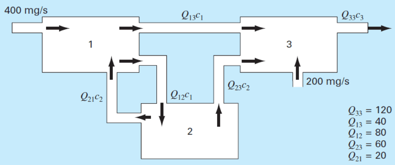
9. Figure below shows three reactors linked by pipes. The mass balance equations for the reactors are shown below:

   For steady state flow: Mass flow rate input $=$ Mass flow rate output

   For example, $400 \mathrm{mg} / \mathrm{s}+Q_{21} c_{2}=Q_{13} c_{1}+Q_{12} c_{1}$ for reactor 1 , where $Q$ is flow rate in $\mathrm{m}^{3} / \mathrm{s}, c$ is concentration of the reactor $\mathrm{mg} / \mathrm{m}^{3}$

   

Continue to develop the linear algebraic equations for the reactors 2 and 3 . Then, solve the concentrations of the reactors by using the Naïve GE.

Solution

$$\begin{aligned} 400+Q_{21} c_2&=Q_{13} c_1+Q_{12} c_1 \\ Q_{12} c_1&=Q_{21} c_2+Q_{23} c_2 \\ Q_{23} c_2+Q_{13} c_1+200&=Q_{33} c_3 \end{aligned}$$

Rearrange:

$$\begin{aligned} 400&=Q_{13} c_1+Q_{12} c_1-Q_{21} c_2 \\ 0&=-Q_{12} c_1+Q_{21} c_2+Q_{23} c_2 \\ 200&=-Q_{13} c_1-Q_{23} c_2+Q_{33} c_3 \end{aligned}$$

$$\begin{aligned} \left[\begin{array}{ccc} Q_{13}+Q_{12} & -Q_{21} & 0 \\ -Q_{12} & Q_{21}+Q_{23} & 0 \\ -Q_{13} & -Q_{23} & Q_{33} \end{array}\right]\left\{\begin{array}{l} c_1 \\ c_2 \\ c_3 \end{array}\right\}&=\left\{\begin{array}{c} 400 \\ 0 \\ 200 \end{array}\right\} \\ \left[\begin{array}{ccc} 40+80 & -20 & 0 \\ -80 & 20+60 & 0 \\ -40 & -60 & 120 \end{array}\right]\left\{\begin{array}{l} c_1 \\ c_2 \\ c_3 \end{array}\right\}&=\left\{\begin{array}{c} 400 \\ 0 \\ 200 \end{array}\right\} \end{aligned}$$

Naïve GE without scaling and partial pivoting, just directly forward elimination and back substitution.

Forward elimination step:

$$\xrightarrow[R3\rightarrow R3-R1(-40/120)]{R2\rightarrow R2-R1(-80/120)} \left[\begin{array}{ccc} 120 & -20 & 0 \\ 0 & 200 / 3 & 0 \\ 0 & -200 / 3 & 120 \end{array}\right]\left\{\begin{array}{l} c_1 \\ c_2 \\ c_3 \end{array}\right\}=\left\{\begin{array}{c} 400 \\ 800 / 3 \\ 1000 / 3 \end{array}\right\}$$

$$\xrightarrow[R3\rightarrow R3-R2(\frac{-200/3}{200/3})]{~} \left[\begin{array}{ccc} 120 & -20 & 0 \\ 0 & 200 / 3 & 0 \\ 0 & 0 & 120 \end{array}\right]\left\{\begin{array}{l} c_1 \\ c_2 \\ c_3 \end{array}\right\}=\left\{\begin{array}{c} 400 \\ 800 / 3 \\ 600 \end{array}\right\}$$

Back substitution step:

$$\begin{gathered} c_3=\frac{600}{120}=5 \\ c_2=\frac{800 / 3}{200 / 3}=4 \\ c_1=\frac{400-(-20) c_2}{120}=4 \\ \left\{\begin{array}{l} c_1 \\ c_2 \\ c_3 \end{array}\right\}=\left\{\begin{array}{l} 4 \\ 4 \\ 5 \end{array}\right\} m g / m^3 \end{gathered}$$

10. Given $z=a_{0}+a_{1} x+a_{2} y$ is a plane equation, where $a$ is the constant coefficient. 3 planes are given below, please suggest a suitable method based on the determinant analysis and continue to find the intersection point/ line of the planes, if it exists.

    

Solution

$$\begin{aligned} 3 x+6 y-3 z&=-6 \\ 4 x-2 y+6 z&=2 \\ 3 x+2 y+z&=-2 \end{aligned}$$

$$\left[\begin{array}{ccc} 3 & 6 & -3 \\ 4 & -2 & 6 \\ 3 & 2 & 1 \end{array}\right]\left\{\begin{array}{l} x \\ y \\ z \end{array}\right\}=\left\{\begin{array}{c} -6 \\ 2 \\ -2 \end{array}\right\}$$

Scaling is important to standardize the matrix before determinant analysis especially for the ill-conditioned case. However, since we don't know the case in the first place, it is important to perform scaling before calculate the determinant

$$\left[\begin{array}{ccc} 3 / 6 & 1 & -3 / 6 \\ 4 / 6 & -2 / 6 & 1 \\ 1 & 2 / 3 & 1 / 3 \end{array}\right]\left\{\begin{array}{l} x \\ y \\ z \end{array}\right\}=\left\{\begin{array}{c} -1 \\ 2 / 6 \\ -2 / 3 \end{array}\right\}$$

Determinant analysis:

$$\left|\begin{array}{ccc} 3 / 6 & 1 & -3 / 6 \\ 4 / 6 & -2 / 6 & 1 \\ 1 & 2 / 3 & 1 / 3 \end{array}\right|=\frac{3}{6}\left(\frac{-2}{18}-\frac{2}{3}\right)-1\left(\frac{4}{18}-1\right)+\left(\frac{-3}{6}\right)\left(\frac{8}{18}+\frac{2}{6}\right)=0$$

Since determinant $=0$, it is singular system where it might have zero solution or infinite solutions.

Matrix inversion method or Cramer's method are not suitable to solve this problem. Thus GEwPP is suggested.

Continue with partial pivoting to reduce the effect of divide by zero issue:

$$\left[\begin{array}{ccc} 1 & 2 / 3 & 1 / 3 \\ 4 / 6 & -2 / 6 & 1 \\ 3 / 6 & 1 & -3 / 6 \end{array}\right]\left\{\begin{array}{l} x \\ y \\ z \end{array}\right\}=\left\{\begin{array}{c} -2 / 3 \\ 2 / 6 \\ -1 \end{array}\right\}$$

Forward elimination

$$\xrightarrow[R 3 \rightarrow R 3-R 1 (3 / 6)]{R 2 \rightarrow R 2-R 1 (4 / 6)} \left[\begin{array}{ccc} 1 & 2 / 3 & 1 / 3 \\ 0 & -7 / 9 & 7 / 9 \\ 0 & 2 / 3 & -2 / 3 \end{array}\right]\left\{\begin{array}{l} x \\ y \\ z \end{array}\right\}=\left\{\begin{array}{c} -2 / 3 \\ 7 / 9 \\ -2 / 3 \end{array}\right\}$$

Pivot element at second row has largest magnitude, thus no partial pivoting is needed.

Forward elimination

$$\xleftarrow[R 3 \rightarrow R 3-R 2 *\left(\frac{2 / 3}{-7 / 9}\right)]{}\left[\begin{array}{ccc} 1 & 2 / 3 & 1 / 3 \\ 0 & -7 / 9 & 7 / 9 \\ 0 & 0 & 0 \end{array}\right]\left\{\begin{array}{l} x \\ y \\ z \end{array}\right\}=\left\{\begin{array}{c} -2 / 3 \\ 7 / 9 \\ 0 \end{array}\right\}$$

Backward substitution

$$0 z=0$$

$Z$ can be any solution, let $z=t,-\infty \leq t \leq \infty$

$$\begin{gathered} y=\frac{\frac{7}{9}-\frac{7}{9} z}{-\frac{7}{9}}=-1+z=-1+t \\ x=\frac{-\frac{2}{3}-\frac{1}{3} z-\frac{2}{3} y}{1}=-\frac{2}{3}-\frac{1}{3} t-\frac{2}{3}(-1+t)=-t \\ \left\{\begin{array}{l} x \\ y \\ z \end{array}\right\}=\left\{\begin{array}{c} -t \\ -1+t \\ t \end{array}\right\} \end{gathered}$$

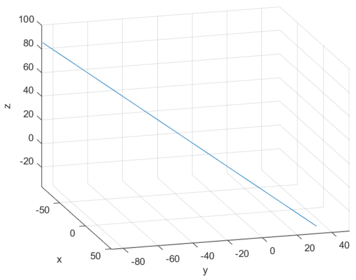
Based on the result, a $3 \mathrm{D}$ line is intersecting all the planes. It can be plotted by using software.

>> t=-100:0.1:100;
>> x=-t;
>> y=-1+t;
>> z=t;
>> xlabel("x")
>> ylabel("y")
>> zlabel("z")

Your Help needed

This website has received 3000 view in the first two weeks! However, this project repository did not receive any star! Just simply head over to this website's repository to give it a star! Every tutorial takes me around two hours to compile, proof-read and styling this website! Your simple action would encourage me a lot! Thank you! You could Buy me a coffee too!