Tutorial 7

Tutorial 7: Matrix Algebra for Homogeneous Linear Algebraic System

Tutorial QuestionTutorial Solution

1. The following linear algebraic equations represents the 3 dof mass spring systems below:

   
   $$\left[\begin{array}{ccc} \frac{k_{1}+k_{2}}{m_{1}} & -\frac{k_{2}}{m_{1}} & 0 \\ -\frac{k_{2}}{m_{2}} & \frac{k_{2}+k_{3}}{m_{2}} & -\frac{k_{3}}{m_{2}} \\ 0 & -\frac{k_{3}}{m_{2}} & \frac{k_{3}+k_{4}}{m_{3}} \end{array}\right]\left\{\begin{array}{l} x_{1} \\ x_{2} \\ x_{3} \end{array}\right\}-\omega^{2}\left[\begin{array}{lll} 1 & 0 & 0 \\ 0 & 1 & 0 \\ 0 & 0 & 1 \end{array}\right]\left\{\begin{array}{l} x_{1} \\ x_{2} \\ x_{3} \end{array}\right\}=\left\{\begin{array}{l} 0 \\ 0 \\ 0 \end{array}\right\}$$

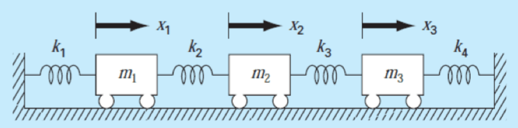
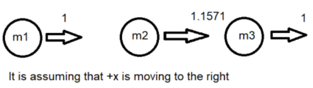
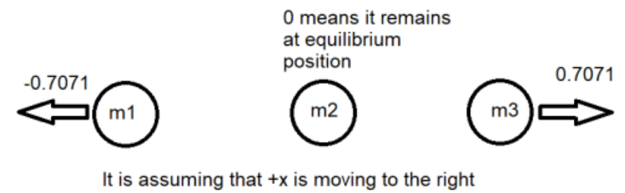
   Determine the smallest eigenvalue and the corresponding eigenvector for the eigenvalue/ eigenvector problem if $k_{1}=k_{4}=15 \frac{N}{m}, k_{2}=k_{3}=35 \frac{N}{m}$, and $m_{1}=m_{2}=$ $m_{3}=1.5 \mathrm{~kg}$. Then, draw the eigenvector.

   Solution

   $$\begin{aligned} \left[\begin{array}{ccc}\frac{k_1+k_2}{m_1} & -\frac{k_2}{m_1} & 0 \\ -\frac{k_2}{m_2} & \frac{k_2+k_3}{m_2} & -\frac{k_3}{m_2} \\ 0 & -\frac{k_3}{m_2} & \frac{k_3+k_4}{m_3}\end{array}\right]\left\{\begin{array}{l}x_1 \\ x_2 \\ x_3\end{array}\right\}-\omega^2\left[\begin{array}{lll}1 & 0 & 0 \\ 0 & 1 & 0 \\ 0 & 0 & 1\end{array}\right]\left\{\begin{array}{l}x_1 \\ x_2 \\ x_3\end{array}\right\}&=\left\{\begin{array}{l}0 \\ 0 \\ 0\end{array}\right\}\\ \left[\begin{array}{ccc}\frac{15+35}{1.5} & -\frac{35}{1.5} & 0 \\ -\frac{35}{1.5} & \frac{35+35}{1.5} & -\frac{35}{1.5} \\ 0 & -\frac{35}{1.5} & \frac{35+15}{1.5}\end{array}\right]\left\{\begin{array}{l}x_1 \\ x_2 \\ x_3\end{array}\right\}-\omega^2\left[\begin{array}{ccc}1 & 0 & 0 \\ 0 & 1 & 0 \\ 0 & 0 & 1\end{array}\right]\left\{\begin{array}{l}x_1 \\ x_2 \\ x_3\end{array}\right\}&=\left\{\begin{array}{l}0 \\ 0 \\ 0\end{array}\right\}\\ \left[\begin{array}{ccc}\frac{100}{3}-\omega^2 & -\frac{70}{3} & 0 \\ -\frac{70}{3} & \frac{140}{3}-\omega^2 & -\frac{70}{3} \\ 0 & -\frac{70}{3} & \frac{100}{3}-\omega^2\end{array}\right]\left\{\begin{array}{l}x_1 \\ x_2 \\ x_3\end{array}\right\}&=\left\{\begin{array}{l}0 \\ 0 \\ 0\end{array}\right\} \end{aligned}$$

   For eigenvalue/eigenvector problem: $\left([A]-\lambda_i[I]\right)\{x\}_i=\{0\}$

   Coefficient matrix, $[A]=\left[\begin{array}{ccc}\frac{100}{3} & -\frac{70}{3} & 0 \\ -\frac{70}{3} & \frac{140}{3} & -\frac{70}{3} \\ 0 & -\frac{70}{3} & \frac{100}{3}\end{array}\right]$

   Eigenvalue, $\lambda=\omega^2$ in this case

   For nontrivial solution, $\left\{\begin{array}{l} x_1 \\ x_2 \\ x_3 \end{array}\right\} \neq\left\{\begin{array}{l} 0 \\ 0 \\ 0 \end{array}\right\}$,

   $$\begin{aligned} \left|\begin{array}{ccc} \frac{100}{3}-\omega^2 & -\frac{70}{3} & 0 \\ -\frac{70}{3} & \frac{140}{3}-\omega^2 & -\frac{70}{3} \\ 0 & -\frac{70}{3} & \frac{100}{3}-\omega^2 \end{array}\right|&=0 \\ \left|\begin{array}{ccc} \frac{100}{3}-\lambda & -\frac{70}{3} & 0 \\ -\frac{70}{3} & \frac{140}{3}-\lambda & -\frac{70}{3} \\ 0 & -\frac{70}{3} & \frac{100}{3}-\lambda \end{array}\right|&=0 \end{aligned}$$

   $$\begin{aligned} 0&=\left(\frac{100}{3}-\lambda\right)\left[\left(\frac{140}{3}-\lambda\right)\left(\frac{100}{3}-\lambda\right)-\left(-\frac{70}{3}\right)\left(-\frac{70}{3}\right)\right]-\left(-\frac{70}{3}\right)\left(\left(-\frac{70}{3}\right)\left(\frac{100}{3}-\lambda\right)\right) \\ 0&=\left(\frac{100}{3}-\lambda\right)\left[\lambda^2-80 t+\frac{9100}{9}\right]+\left[\frac{4900}{9} t-\frac{490000}{27}\right] \\ 0&=\left[-\lambda^3+\frac{340}{3} \lambda^2-\frac{33100}{9} t+\frac{910000}{27}\right]+\left[\frac{4900}{9} t-\frac{490000}{27}\right] \\ 0&=-\lambda^3+\frac{340}{3} \lambda^2-\frac{9400}{3} \lambda+\frac{140000}{9} \end{aligned}$$

   Using calculator or software:

   >> polynomial = [-1 340/3 -9400/3 140000/9]
   >> root=roots(polynomial)

   $$\begin{aligned} \lambda_1&=\frac{3839}{606}=6.3350 \\ \lambda_2&=\frac{100}{3}=33.3333 \\ \lambda_3&=\frac{14954}{203}=73.6650 \end{aligned}$$

   For case 1 $\left(\lambda_1=\frac{3839}{606}=6.3350=\omega_1^2\right)$:

   $$\begin{aligned} \begin{bmatrix}\frac{100}{3}-\frac{3839}{606} & -\frac{70}{3} & 0 \\ -\frac{70}{3} & \frac{140}{3}-\frac{3839}{606} & -\frac{70}{3} \\ 0 & -\frac{70}{3} & \frac{100}{3}-\frac{3839}{606}\end{bmatrix}\left\{\begin{array}{l}x_1 \\ x_2 \\ x_3\end{array}\right\}_1&=\left\{\begin{array}{l}0 \\ 0 \\ 0\end{array}\right\}\\ \begin{bmatrix}\frac{16361}{606} & -\frac{70}{3} & 0 \\ -\frac{70}{3} & \frac{8147}{202} & -\frac{70}{3} \\ 0 & -\frac{70}{3} & \frac{16361}{606}\end{bmatrix}\left\{\begin{array}{l}x_1 \\ x_2 \\ x_3\end{array}\right\}_1&=\left\{\begin{array}{l}0 \\ 0 \\ 0\end{array}\right\}\\ \xrightarrow[R1\rightarrow R1\left(\frac{606}{16361}\right)]{} \left[\begin{array}{ccc}1 & -\frac{1216}{1407} & 0 \\ -\frac{70}{3} & \frac{8147}{202} & -\frac{70}{3} \\ 0 & -\frac{70}{3} & \frac{16361}{606}\end{array}\right]\left\{\begin{array}{l}x_1 \\ x_2 \\ x_3\end{array}\right\}_1&=\left\{\begin{array}{l}0 \\ 0 \\ 0\end{array}\right\}\\ \xrightarrow[R2\rightarrow R2-R1\left(\frac{-70}{3}\right)]{} \left[\begin{array}{ccc}1 & -\frac{1216}{1407} & 0 \\ 0 & \frac{4134}{205} & -\frac{70}{3} \\ 0 & -\frac{70}{3} & \frac{16361}{606}\end{array}\right]\left\{\begin{array}{l}x_1 \\ x_2 \\ x_3\end{array}\right\}_1&=\left\{\begin{array}{l}0 \\ 0 \\ 0\end{array}\right\}\\ \xrightarrow[R2\rightarrow R2\left(\frac{205}{4134}\right)]{} \left[\begin{array}{ccc}1 & -\frac{1216}{1407} & 0 \\ 0 & 1 & -\frac{1849}{1598} \\ 0 & -\frac{70}{3} & \frac{16361}{606}\end{array}\right]\left\{\begin{array}{l}x_1 \\ x_2 \\ x_3\end{array}\right\}_1&=\left\{\begin{array}{l}0 \\ 0 \\ 0\end{array}\right\}\\ \xrightarrow[R3\rightarrow R3-R2\left(\frac{-70}{3}\right)]{} \left[\begin{array}{ccc}1 & -\frac{1216}{1407} & 0 \\ 0 & 1 & -\frac{1849}{1598} \\ 0 & 0 & \mathbf{0} \end{array}\right]\left\{\begin{array}{l}x_1 \\ x_2 \\ x_3\end{array}\right\}_1&=\left\{\begin{array}{l}0 \\ 0 \\ 0\end{array}\right\}\\ \xrightarrow[R1\rightarrow R1-R2\left(\frac{-1216}{1407}\right)]{} \left[\begin{array}{ccc}1 & 0 & -1 \\ 0 & 1 & -\frac{1849}{1598} \\ 0 & 0 & \mathbf{0} \end{array}\right]\left\{\begin{array}{l}x_1 \\ x_2 \\ x_3\end{array}\right\}_1&=\left\{\begin{array}{l}0 \\ 0 \\ 0\end{array}\right\}\\ \end{aligned}$$

   Note: RREF shows rank 2 (i.e. 2 linearly independent vectors)

   $x_1-x_3=0 \gg x_1=x_3$

   $x_2-\frac{1849}{1598} x_3=0 \gg x_2=\frac{1849}{1598} x_3$

   Eigenspace for $\left\{\begin{array}{l} x_1 \\ x_2 \\ x_3 \end{array}\right\}_{\lambda=6.3350}=\left\{\begin{array}{c} x_3 \\ \frac{1849}{1598} x_3 \end{array}\right\}=\left.t\left\{\begin{array}{c} 1849 \\ 1598 \\ 1 \end{array}\right\}\right|_{x_3=t}$, where $t\in \mathbb{R}$

   Eigenvector, $\left\{\begin{array}{l} x_1 \\ x_2 \\ x_3 \end{array}\right\}_{\lambda=6.3350}=\left\{\begin{array}{c} 1 \\ 1.1571 \\ 1 \end{array}\right\}$

   

2. Continue from Q1, determine the second largest eigenvalue and the corresponding normalised eigenvector. Then, draw the eigenvector.

   Solution

   For case 2 $\left(\lambda_2=\frac{100}{3}=33.3333=\omega_2^2\right)$:

   $$\begin{aligned} \left[\begin{array}{ccc} \frac{100}{3}-\frac{100}{3} & -\frac{70}{3} & 0 \\ -\frac{70}{3} & \frac{140}{3}-\frac{100}{3} & -\frac{70}{3} \\ 0 & -\frac{70}{3} & \frac{100}{3}-\frac{100}{3} \end{array}\right]\left\{\begin{array}{l} x_1 \\ x_2 \\ x_3 \end{array}\right\}_2&=\left\{\begin{array}{l} 0 \\ 0 \\ 0 \end{array}\right\}\\ \left[\begin{array}{ccc} 0 & -\frac{70}{3} & 0 \\ -\frac{70}{3} & \frac{40}{3} & -\frac{70}{3} \\ 0 & -\frac{70}{3} & 0 \end{array}\right]\left\{\begin{array}{l} x_1 \\ x_2 \\ x_3 \end{array}\right\}_2&=\left\{\begin{array}{l} 0 \\ 0 \\ 0 \end{array}\right\}\\ \xrightarrow[R 1 \leftrightarrow R 2]{}\left[\begin{array}{ccc} -\frac{70}{3} & \frac{40}{3} & -\frac{70}{3} \\ 0 & -\frac{70}{3} & 0 \\ 0 & -\frac{70}{3} & 0 \end{array}\right]\left\{\begin{array}{l} x_1 \\ x_2 \\ x_3 \end{array}\right\}_2&=\left\{\begin{array}{l} 0 \\ 0 \\ 0 \end{array}\right\}\\ \xrightarrow[R 1 \rightarrow R 1 (-3 / 70)]{} \left[\begin{array}{ccc} 1 & \frac{-4}{7} & 1 \\ 0 & -\frac{70}{3} & 0 \\ 0 & -\frac{70}{3} & 0 \end{array}\right]\left\{\begin{array}{l} x_1 \\ x_2 \\ x_3 \end{array}\right\}_2&=\left\{\begin{array}{l} 0 \\ 0 \\ 0 \end{array}\right\}\\ \xrightarrow[R 2 \rightarrow R 2 (-3 / 70)]{} \left[\begin{array}{ccc} 1 & \frac{-4}{7} & 1 \\ 0 & 1 & 0 \\ 0 & -\frac{70}{3} & 0 \end{array}\right]\left\{\begin{array}{l} x_1 \\ x_2 \\ x_3 \end{array}\right\}_2&=\left\{\begin{array}{l} 0 \\ 0 \\ 0 \end{array}\right\}\\ \xrightarrow[R 3 \rightarrow R 3 - R 2 (-70 / 3)]{} \left[\begin{array}{ccc} 1 & \frac{-4}{7} & 1 \\ 0 & 1 & 0 \\ 0 & 0 & 0 \end{array}\right]\left\{\begin{array}{l} x_1 \\ x_2 \\ x_3 \end{array}\right\}_2&=\left\{\begin{array}{l} 0 \\ 0 \\ 0 \end{array}\right\}\\ \xrightarrow[R 1 \rightarrow R 1 - R 2 (-4 / 7)]{} \left[\begin{array}{ccc} 1 & 0 & 1 \\ 0 & 1 & 0 \\ 0 & 0 & 0 \end{array}\right]\left\{\begin{array}{l} x_1 \\ x_2 \\ x_3 \end{array}\right\}_2&=\left\{\begin{array}{l} 0 \\ 0 \\ 0 \end{array}\right\} \end{aligned}$$

   Note: RREF shows rank 2 (i.e 2 linearly independent vectors)

   $x_1+x_3=0\gg x_1=-x_3$

   $x_2=0$

   Eigenspace for $\left\{\begin{array}{l}x_1 \\ x_2 \\ x_3\end{array}\right\}_{\lambda=33.3333}=\left\{\begin{array}{c}-x_3 \\ 0 \\ x_3\end{array}\right\}=\left.t\left\{\begin{array}{c}-1 \\ 0 \\ 1\end{array}\right\}\right|_{x_3=t}$, where $t \in \mathbb{R}$

   Note: If it is not specific the type of eigenvector, normally unscaled eigenvector by let $t=1$ is provided for manual calculation.

   Eigenvector, $\left\{\begin{array}{l}x_1 \\ x_2 \\ x_3\end{array}\right\}_{\lambda=33.3333}=\left\{\begin{array}{c}-1 \\ 0 \\ 1\end{array}\right\}$

   Normalised Eigenvector, $\left\{\begin{array}{l}x_1 \\ x_2 \\ x_3\end{array}\right\}_{\lambda=33.3333, \text { normalised }}=\frac{1}{\sqrt{2}}\left\{\begin{array}{c}-1 \\ 0 \\ 1\end{array}\right\}=\left\{\begin{array}{c}-0.7071 \\ 0 \\ 0.7071\end{array}\right\}$

   

3. Continue from Q1, determine the largest eigenvalue and the corresponding unscaled eigenvector. Then, draw the eigenvector.

   Solution

   $$\begin{aligned} \left[\begin{array}{ccc} \frac{100}{3}-\frac{14954}{203} & -\frac{70}{3} & 0 \\ -\frac{70}{3} & \frac{140}{3}-\frac{14954}{203} & -\frac{70}{3} \\ 0 & -\frac{70}{3} & \frac{100}{3}-\frac{14954}{203} \end{array}\right]\left\{\begin{array}{l} x_1 \\ x_2 \\ x_3 \end{array}\right\}_3&=\left\{\begin{array}{l} 0 \\ 0 \\ 0 \end{array}\right\} \\ \left[\begin{array}{ccc} \frac{-8147}{202} & -\frac{70}{3} & 0 \\ -\frac{70}{3} & \frac{-16442}{609} & -\frac{70}{3} \\ 0 & -\frac{70}{3} & \frac{-8147}{202} \end{array}\right]\left\{\begin{array}{l} x_1 \\ x_2 \\ x_3 \end{array}\right\}&=\left\{\begin{array}{l} 0 \\ 0 \\ 0 \end{array}\right\}\\ \xrightarrow[R1\rightarrow R1(-202/8147)]{} \left[\begin{array}{ccc} 1 & \frac{814}{1407} & 0 \\ -\frac{70}{3} & \frac{-16442}{609} & -\frac{70}{3} \\ 0 & -\frac{70}{3} & \frac{-8147}{202} \end{array}\right]\left\{\begin{array}{l} x_1 \\ x_2 \\ x_3 \end{array}\right\}_3&=\left\{\begin{array}{l} 0 \\ 0 \\ 0 \end{array}\right\} \\ \xrightarrow[R2\rightarrow R2-R1(-70/3)]{} \left[\begin{array}{ccc} 1 & \frac{814}{1407} & 0 \\ 0 & \frac{-8302}{615} & -\frac{70}{3} \\ 0 & -\frac{70}{3} & \frac{-8147}{202} \end{array}\right]\left\{\begin{array}{l} x_1 \\ x_2 \\ x_3 \end{array}\right\}_3&=\left\{\begin{array}{l} 0 \\ 0 \\ 0 \end{array}\right\} \\ \xrightarrow[R2\rightarrow R2(-615/8302)]{} \left[\begin{array}{ccc} 1 & \frac{814}{1407} & 0 \\ 0 & 1 & \frac{1025}{593} \\ 0 & -\frac{70}{3} & \frac{-8147}{202} \end{array}\right]\left\{\begin{array}{l} x_1 \\ x_2 \\ x_3 \end{array}\right\}_3&=\left\{\begin{array}{l} 0 \\ 0 \\ 0 \end{array}\right\} \\ \xrightarrow[R3\rightarrow R3-R2(-70/3)]{} \left[\begin{array}{ccc} 1 & \frac{814}{1407} & 0 \\ 0 & 1 & \frac{1025}{593} \\ 0 & 0 & \mathbf{0} \\ \end{array}\right]\left\{\begin{array}{l} x_1 \\ x_2 \\ x_3 \end{array}\right\}_3&=\left\{\begin{array}{l} 0 \\ 0 \\ 0 \end{array}\right\} \\ \xrightarrow[R1\rightarrow R1-R2(814/1407)]{} \left[\begin{array}{ccc} 1 & 0 & -1 \\ 0 & 1 & \frac{1025}{593} \\ 0 & 0 & \mathbf{0} \\ \end{array}\right]\left\{\begin{array}{l} x_1 \\ x_2 \\ x_3 \end{array}\right\}_3&=\left\{\begin{array}{l} 0 \\ 0 \\ 0 \end{array}\right\} \\ \end{aligned}$$

   Note: RREF shows rank 2 (i.e. 2 linearly independent vectors)

   $x_1-x_3=0 \gg x_1=x_3$

   $x_2+\frac{1025}{593} x_3=0 \gg x_2=-\frac{1025}{593} x_3$

   Eigenspace for $\left\{\begin{array}{l} x_1 \\ x_2 \\ x_3 \end{array}\right\}_{\lambda=73.6650}=\left\{\begin{array}{c} x_3 \\ -\frac{1025}{593} x_3 \\ x_3 \end{array}\right\}=\left.t\left\{\begin{array}{c} 1 \\ -\frac{1025}{593} \\ 1 \end{array}\right\}\right|_{x_3=t}$, where $t\in\mathbb{R}$

   Note: Unscaled eigenvectors can be any vector of eigenspace. Normally we just let $t=1$

   Eigenvector, $\left\{\begin{array}{l}x_1 \\ x_2 \\ x_3\end{array}\right\}_{\lambda=73.6650}=\left\{\begin{array}{c}1 \\ -1.7285 \\ 1\end{array}\right\}$

   

4. Combining the results obtained from Q1-Q4, obtain the eigenvector matrix, $P$ and diagonalize the following matrix. Comment the relationship between the diagonal matrix and the eigenvalue.

   $$\left[\begin{array}{ccc} \frac{k_{1}+k_{2}}{m_{1}} & -\frac{k_{2}}{m_{1}} & 0 \\ -\frac{k_{2}}{m_{2}} & \frac{k_{2}+k_{3}}{m_{2}} & -\frac{k_{3}}{m_{2}} \\ 0 & -\frac{k_{3}}{m_{2}} & \frac{k_{3}+k_{4}}{m_{3}} \end{array}\right]$$
   Solution

   $$\mathbf{A}=\left[\begin{array}{ccc} \frac{100}{3} & -\frac{70}{3} & 0 \\ -\frac{70}{3} & \frac{140}{3} & -\frac{70}{3} \\ 0 & -\frac{70}{3} & \frac{100}{3} \end{array}\right] \mathbf{P}=\left[\begin{array}{ccc} 1 & -0.7071 & 1 \\ 1.1571 & 0 & -1.7285 \\ 1 & 0.7071 & 1 \end{array}\right]$$

   Diagonal matrix, $\mathbf{D}=\mathbf{P}^{\mathbf{- 1}} \mathbf{A P}$

   $$\mathbf{P}^{-\mathbf{1}}=\frac{\mathbf{1}}{\operatorname{det}(\mathbf{P})} \operatorname{adjoint}(\mathbf{P})$$

   $$\begin{aligned} \operatorname{cofactor}(\mathbf{P})&=\begin{bmatrix} \left|\begin{matrix} 0&-1.7285\\-1.7285&1 \end{matrix}\right| & -\left|\begin{matrix} 1.1571&-1.7285\\1&1 \end{matrix}\right| & -\left|\begin{matrix} 1.1571&0\\1&0.7071 \end{matrix}\right|\\ -\left|\begin{matrix} -0.7071&1\\0.7071&1 \end{matrix}\right| & -\left|\begin{matrix} 1&1\\1&1 \end{matrix}\right| & -\left|\begin{matrix} 1&-0.7071\\1&0.7071 \end{matrix}\right|\\ \left|\begin{matrix} -0.7071&1\\0&-1.7285 \end{matrix}\right| & \left|\begin{matrix} 1&1\\1.1571&-1.7285 \end{matrix}\right| & \left|\begin{matrix} 1&-0.7071\\1.1571&0 \end{matrix}\right| \end{bmatrix}\\ &=\begin{bmatrix} 1.2222&1.4142&1.2222\\ -2.8856&0&2.8856\\ 0.8182&-1.4142&0.8182 \end{bmatrix} \end{aligned}$$

   $\operatorname{adjoint}(\mathbf{P})=\left[\begin{array}{ccc}1.2222 & -2.8856 & 0.8182 \\ 1.4142 & 0 & -1.4142 \\ 1.2222 & 2.8856 & 0.8182\end{array}\right]$

   $$\begin{aligned} \operatorname{det}(\mathbf{P})&=\left|\begin{array}{ccc}1 & -0.7071 & 1 \\ 1.1571 & 0 & -1.7285 \\ 1 & 0.7071 & 1\end{array}\right|\\ &=-(-1.7285)(0.7071)-(-0.7071)(1.1571+1.7285)+(1.1571)(0.7071)\\ &=4.0808 \end{aligned}$$

   $$\mathbf{P}^{-1}=\frac{1}{4.0808}\left[\begin{array}{ccc} 1.2222 & -2.8856 & 0.8182 \\ 1.4142 & 0 & -1.4142 \\ 1.2222 & 2.8856 & 0.8182 \end{array}\right]=\left[\begin{array}{ccc} 0.2995 & 0.3465 & 0.2995 \\ -0.7071 & 0 & 0.7071 \\ 0.2005 & -0.3465 & 0.2005 \end{array}\right]$$

   $$\begin{aligned} D&=P^{-1} A P\\ &=\left[\begin{array}{ccc} 0.2995 & 0.3465 & 0.2995 \\ -0.7071 & 0 & 0.7071 \\ 0.2005 & -0.3465 & 0.2005 \end{array}\right]\left[\begin{array}{ccc} \frac{100}{3} & -\frac{70}{3} & 0 \\ -\frac{70}{3} & \frac{140}{3} & -\frac{70}{3} \\ 0 & -\frac{70}{3} & \frac{100}{3} \end{array}\right]\left[\begin{array}{ccc} 1 & -0.7071 & 1 \\ 1.1571 & 0 & -1.7285 \\ 1 & 0.7071 & 1 \end{array}\right]\\ &=\left[\begin{array}{ccc} 1.8974 & 2.1954 & 1.8974 \\ -23.5705 & 0 & 23.5705 \\ 14.7693 & -25.5287 & 14.7693 \end{array}\right]\left[\begin{array}{ccc} 1 & -0.7071 & 1 \\ 1.1571 & 0 & -1.7285 \\ 1 & 0.7071 & 1 \end{array}\right]\\ &=\left[\begin{array}{ccc} 6.335 & 0 & 0 \\ 0 & 33.3333 & 0 \\ 0 & 0 & 73.665 \end{array}\right] \quad ; \quad \mathbf{D}=\left[\begin{array}{ccc} \lambda_1 & 0 & 0 \\ 0 & \lambda_2 & 0 \\ 0 & 0 & \lambda_3 \end{array}\right] \end{aligned}$$

5. Determine $\left[\begin{array}{ccc}\frac{k_{1}+k_{2}}{m_{1}} & -\frac{k_{2}}{m_{1}} & 0 \\ -\frac{k_{2}}{m_{2}} & \frac{k_{2}+k_{3}}{m_{2}} & -\frac{k_{3}}{m_{2}} \\ 0 & -\frac{k_{3}}{m_{2}} & \frac{k_{3}+k_{4}}{m_{3}}\end{array}\right]^{50}$ and comment on the change of it's eigenvalue and eigenvector, as compared to $\mathrm{Q} 4$.

   Solution

   $$\begin{aligned} &\left[\begin{array}{ccc}\frac{k_1+k_2}{m_1} & -\frac{k_2}{m_1} & 0 \\ -\frac{k_2}{m_2} & \frac{k_2+k_3}{m_2} & -\frac{k_3}{m_2} \\ 0 & -\frac{k_3}{m_2} & \frac{k_3+k_4}{m_3}\end{array}\right]^{50}=\mathbf{A}^{50}=\mathbf{P D}^{50} \mathbf{P}^{-1}\\ &=\left[\begin{array}{ccc}\frac{100}{3} & -\frac{70}{3} & 0 \\ -\frac{70}{3} & \frac{140}{3} & -\frac{70}{3} \\ 0 & -\frac{70}{3} & \frac{100}{3}\end{array}\right]\left[\begin{array}{ccccc}6.335 & 0 & 0 \\ 0 & 33.3333 & 0 \\ 0 & 0 & 73.665\end{array}\right]^{50}\left[\begin{array}{ccc}0.2995 & 0.3465 & 0.2995 \\ -0.7071 & 0 & 0.7071 \\ 0.2005 & -0.3465 & 0.2005\end{array}\right]\\ &=\left[\begin{array}{ccc}\frac{100}{3} & -\frac{70}{3} & 0 \\ -\frac{70}{3} & \frac{140}{3} & -\frac{70}{3} \\ 0 & -\frac{70}{3} & \frac{100}{3}\end{array}\right]\left[\begin{array}{ccc}6.335^{50} & 0 & 0 \\ 0 & 33.3333^{50} & 0 \\ 0 & 0 & 73.665^{50}\end{array}\right]\left[\begin{array}{ccc}0.2995 & 0.3465 & 0.2995 \\ -0.7071 & 0 & 0.7071 \\ 0.2005 & -0.3465 & 0.2005\end{array}\right]\\ &=\left[\begin{array}{ccc}\frac{100}{3} & -\frac{70}{3} & 0 \\ -\frac{70}{3} & \frac{140}{3} & -\frac{70}{3} \\ 0 & -\frac{70}{3} & \frac{100}{3}\end{array}\right]\left[\begin{array}{ccccc}6.335^{50} & 0 & 0 \\ 0 & 33.3333^{50} & 0 \\ 0 & 0 & 73.665^{50}\end{array}\right]\left[\begin{array}{ccc}0.2995 & 0.3465 & 0.2995 \\ -0.7071 & 0 & 0.7071 \\ 0.2005 & -0.3465 & 0.2005\end{array}\right]\\ &=10^{93}\left[\begin{array}{llc}-0.00002228 & 0.00000000 & 2.30708930 \\ -0.00003851 & 0.00000000 & -3.98780548 \\ -0.00002228 & 0.00000000 & 2.30708930\end{array}\right]\left[\begin{array}{ccc}0.2995 & 0.3465 & 0.2995 \\ -0.7071 & 0 & 0.7071 \\ 0.2005 & -0.3465 & 0.2005\end{array}\right]\\ &=10^{93}\left[\begin{array}{ccc}0.46255450 & -0.79952578 & 0.46255450 \\ -0.79952578 & 1.38198087 & -0.79952578 \\ 0.46255450 & -0.79952578 & 0.46255450\end{array}\right] \end{aligned}$$

   Eigenvalue $(\mathbf{A}^{50})=\lambda_i^{50}$, where $k\in\mathbf{R}$. It means the eigenvalue is power of 50 higher than the original eigenvalue. The eigenvector of $\mathbf{A}^{50}$ and $\mathbf{A}$ remains unchanged.

6. Given $\mathbf{B}=\left[\begin{array}{lll}1 & 2 & 3 \\ 0 & 1 & 1 \\ 0 & 0 & 2\end{array}\right]$ and $|\mathbf{B}|=2$ has an eigenvalue of 2 . Find the remaining eigenvalues and develop the characteristic equation without developing the eigenvalue problem and without performing the determinant.

   Solution

   $\mathbf{B}=\left[\begin{array}{lll} 1 & 2 & 3 \\ 0 & 1 & 1 \\ 0 & 0 & 2 \end{array}\right]$

   $|\mathbf{B}|=2$ has an eigenvalue of 2

   $\mathbf{B}$ has 3 eigenvalues since it has $3 \times 3$ matrix.

   From the property,

   $$\begin{aligned} \operatorname{Trace}(\mathbf{B})&=\sum \lambda_i=\lambda_1+\lambda_2+\lambda_3\\ 1+1+2&=\lambda_1+\lambda_2+(2) \\ \lambda_1+\lambda_2&=2 \end{aligned} \tag{1}$$

   From the property,

   $$\begin{aligned} \operatorname{Determinant}(\mathbf{A})&=\prod \lambda_i=\lambda_1 \lambda_2 \lambda_3\\ 2&=\lambda_1 \lambda_2(2) \\ \lambda_1 \lambda_2&=1 \end{aligned} \tag{2}$$

   Subs (2) into (1)

   $$\begin{aligned} \lambda_1+\frac{1}{\lambda_1}&=2 \\ \lambda_1^2-2 \lambda_1+1&=0 \\ \left(\lambda_1-1\right)^2&=0 \\ \lambda_1&=1 \\ \lambda_2&=\frac{1}{\lambda_1}=1 \end{aligned}$$

   $\therefore \lambda_1=1, \lambda_2=1, \lambda_3=2$

   Characteristic equation:

   $$\begin{aligned} (\lambda-1)(\lambda-1)(\lambda-2)&=0 \\ \left(\lambda^2-2 \lambda+1\right)(\lambda-2)&=0\\ \lambda^3+(-4) \lambda^2+(5) \lambda-2&=0 \end{aligned}$$

7. Continue Q6, using Cayley-Hamilton theorem to verify that:

   $\mathbf{B}^{-1}=\frac{1}{2} \mathbf{B}^{2}+(-2) \mathbf{B}+\left(\frac{5}{2}\right) \mathbf{I}$ and $\mathbf{B}^{6}=\left[(57) \mathbf{B}^{2}+(-108) \mathbf{B}+52 \mathbf{I}\right]$. Then, compute the $\mathbf{B}^{5}$ via the theorem.

   Solution

   $$\begin{aligned} \mathbf{B}^3+(-4) \mathbf{B}^2+(5) \mathbf{B}-2 \mathbf{I}&=\mathbf{0}\\ \mathbf{B}^2+(-4) \mathbf{B}+(5) \mathbf{I}-2 \mathbf{B}^{-1}&=\mathbf{0}\\ \mathbf{B}^{-1}&=\frac{1}{2} \mathbf{B}^2+(-2) \mathbf{B}+\left(\frac{5}{2}\right) \mathbf{I} \quad\text { (verified) }\\\\ \mathbf{B}^4+(-4) \mathbf{B}^3+(5) \mathbf{B}^2-2 \mathbf{B}&=\mathbf{0}\\ \mathbf{B}^4&=(4) \mathbf{B}^3-(5) \mathbf{B}^2+2 \mathbf{B}\\ \mathbf{B}^4&=\left[(16) \mathbf{B}^2-(20) \mathbf{B}+8 \mathbf{I}\right]-(5) \mathbf{B}^2+2 \mathbf{B}\\ \mathbf{B}^4&=\left[(11) \mathbf{B}^2-(18) \mathbf{B}+8 \mathbf{I}\right]\\ \mathbf{B}^5&=(11) \mathbf{B}^3-(18) \mathbf{B}^2+8 \mathbf{B}\\ \mathbf{B}^5&=\left[(44) \mathbf{B}^2-(55) \mathbf{B}+22 \mathbf{I}\right]-(18) \mathbf{B}^2+8 \mathbf{B}\\ \mathbf{B}^5&=(26) \mathbf{B}^2-(47) \mathbf{B}+22 \mathbf{I}\\ \mathbf{B}^6&=(26) \mathbf{B}^3-(47) \mathbf{B}^2+22 \mathbf{B}\\ \mathbf{B}^6&=\left[(104) \mathbf{B}^2+(-130) \mathbf{B}+52 \mathbf{I}\right]-(47) \mathbf{B}^2+22 \mathbf{B}\\ \mathbf{B}^6&=\left[(57) \mathbf{B}^2+(-108) \mathbf{B}+52 \mathbf{I}\right] \quad\text { (verified) }\\ \end{aligned}$$

   $$\mathbf{B}=\left[\begin{array}{lll} 1 & 2 & 3 \\ 0 & 1 & 1 \\ 0 & 0 & 2 \end{array}\right]$$

   $$\begin{aligned} \mathbf{B}^5&=(26) \mathbf{B}^2-(47) \mathbf{B}+22 \mathbf{I}\\ &=(26)\left[\begin{array}{lll} 1 & 2 & 3 \\ 0 & 1 & 1 \\ 0 & 0 & 2 \end{array}\right]\left[\begin{array}{lll} 1 & 2 & 3 \\ 0 & 1 & 1 \\ 0 & 0 & 2 \end{array}\right]-(47)\left[\begin{array}{lll} 1 & 2 & 3 \\ 0 & 1 & 1 \\ 0 & 0 & 2 \end{array}\right]+22\left[\begin{array}{lll} 1 & 0 & 0 \\ 0 & 1 & 0 \\ 0 & 0 & 1 \end{array}\right]\\ &=(26)\left[\begin{array}{lcc} 1 & 4 & 11 \\ 0 & 1 & 3 \\ 0 & 0 & 4 \end{array}\right]-(47)\left[\begin{array}{lll} 1 & 2 & 3 \\ 0 & 1 & 1 \\ 0 & 0 & 2 \end{array}\right]+22\left[\begin{array}{lll} 1 & 0 & 0 \\ 0 & 1 & 0 \\ 0 & 0 & 1 \end{array}\right]\\ &=\left[\begin{array}{ccc} 1 & 10 & 145 \\ 0 & 1 & 31 \\ 0 & 0 & 32 \end{array}\right] \end{aligned}$$

8. Explain why the following equation : $\mathbf{B}^{5}=\mathbf{P D}^{5} \mathbf{P}^{-1}$ is not working to solve the $Q 7$ problem?

   Solution

   Previously we obtained,

   $$\mathbf{B}=\left[\begin{array}{lll} 1 & 2 & 3 \\ 0 & 1 & 1 \\ 0 & 0 & 2 \end{array}\right]$$

   $\lambda_1=1, \lambda_2=1, \lambda_3=2$

   where $\mathbf{D}=\left[\begin{array}{lll}1 & 0 & 0 \\ 0 & 1 & 0 \\ 0 & 0 & 2\end{array}\right]$

   The eigenvalue/eigenvector problem: $(\mathbf{B}-\lambda \mathbf{I}) x=\mathbf{0}$

   For $\lambda_1=1$

   $$\begin{aligned} \left[\begin{array}{ccc}1-1 & 2 & 3 \\ 0 & 1-1 & 1 \\ 0 & 0 & 2-1\end{array}\right]\left\{\begin{array}{l}x_1 \\ x_2 \\ x_3\end{array}\right\}_1&=\left\{\begin{array}{l}0 \\ 0 \\ 0\end{array}\right\}\\ \left[\begin{array}{lll}0 & 2 & 3 \\ 0 & 0 & 1 \\ 0 & 0 & 1\end{array}\right]\left\{\begin{array}{l}x_1 \\ x_2 \\ x_3\end{array}\right\}_1&=\left\{\begin{array}{l}0 \\ 0 \\ 0\end{array}\right\}\\ \xrightarrow[R1\rightarrow R1(1/2)]{} \left[\begin{array}{lll}0 & 1 & 3/2 \\ 0 & 0 & 1 \\ 0 & 0 & 1\end{array}\right]\left\{\begin{array}{l}x_1 \\ x_2 \\ x_3\end{array}\right\}_1&=\left\{\begin{array}{l}0 \\ 0 \\ 0\end{array}\right\}\\ \xrightarrow[R1\rightarrow R1-R2(3/2)]{R3\rightarrow R3-R2(1)} \left[\begin{array}{lll}0 & 1 & 0 \\ 0 & 0 & 1 \\ 0 & 0 & 0\end{array}\right]\left\{\begin{array}{l}x_1 \\ x_2 \\ x_3\end{array}\right\}_1&=\left\{\begin{array}{l}0 \\ 0 \\ 0\end{array}\right\}\\ \end{aligned}$$

   Note: RREF shows rank 2 (i.e. 2 linearly independent vectors)

   $x_2=0$ $x_3=0$

   Eigenspace for $\left\{\begin{array}{l}x_1 \\ x_2 \\ x_3\end{array}\right\}_{\lambda=1}=\left\{\begin{array}{l}x_1 \\ 0 \\ 0\end{array}\right\}=\left.t\left\{\begin{array}{l}1 \\ 0 \\ 0\end{array}\right\}\right|_{x_1=t}$, where $t \in \mathbb{R}$

   Note: Unscaled eigenvectors can be any vector of eigenspace. Normally we just let $t=1$

   Eigenvector, $\left\{\begin{array}{l}x_1 \\ x_2 \\ x_3\end{array}\right\}_{\lambda=1}=\left\{\begin{array}{l}1 \\ 0 \\ 0\end{array}\right\}$

   For repeated eigenvalue, $\lambda_2=1$

   Eigenvector, $\left\{\begin{array}{l}x_1 \\ x_2 \\ x_3\end{array}\right\}_{\lambda=1}=\left\{\begin{array}{l}1 \\ 0 \\ 0\end{array}\right\}$

   For $\lambda_3=2$

   $$\begin{aligned} \left[\begin{array}{ccc}1-2 & 2 & 3 \\ 0 & 1-2 & 1 \\ 0 & 0 & 2-2\end{array}\right]\left\{\begin{array}{l}x_1 \\ x_2 \\ x_3\end{array}\right\}&=\left\{\begin{array}{l}0 \\ 0 \\ 0\end{array}\right\}\\ \left[\begin{array}{ccc}-1 & 2 & 3 \\ 0 & -1 & 1 \\ 0 & 0 & 0\end{array}\right]\left\{\begin{array}{l}x_1 \\ x_2 \\ x_3\end{array}\right\}_3&=\left\{\begin{array}{l}0 \\ 0 \\ 0\end{array}\right\} \end{aligned}$$

   $$\begin{aligned} \xrightarrow[R2\rightarrow R2(-1)]{R1\rightarrow R1(-1)} \left[\begin{array}{ccc} 1 & -2 & -3 \\ 0 & 1 & -1 \\ 0 & 0 & 0\end{array}\right]\left\{\begin{array}{l}x_1 \\ x_2 \\ x_3\end{array}\right\}_3&=\left\{\begin{array}{l}0 \\ 0 \\ 0\end{array}\right\}\\ \xrightarrow[R1\rightarrow R1-R2(-2)]{} \left[\begin{array}{ccc} 1 & 0 & -5 \\ 0 & 1 & -1 \\ 0 & 0 & 0\end{array}\right]\left\{\begin{array}{l}x_1 \\ x_2 \\ x_3\end{array}\right\}_3&=\left\{\begin{array}{l}0 \\ 0 \\ 0\end{array}\right\} \end{aligned}$$

   Note: RREF shows rank 2 (i.e. 2 linearly independent vectors)

   $x_1-5 x_3=0 \gg x_1=5 x_3$ $x_2-x_3=0 \gg x_2=x_3$

   Eigenspace for $\left\{\begin{array}{l} x_1 \\ x_2 \\ x_3 \end{array}\right\}_{\lambda=2}=\left\{\begin{array}{c} 5 x_3 \\ x_3 \\ x_3 \end{array}\right\}=\left.t\left\{\begin{array}{l} 5 \\ 1 \\ 1 \end{array}\right\}\right|_{x_3=t}$ , where $t\in\mathbb{R}$

   Note: Unscaled eigenvectors can be any vector of eigenspace. Normally we just let $t=1$

   Eigenvector, $\left\{\begin{array}{l}x_1 \\ x_2 \\ x_3\end{array}\right\}_{\lambda=2}=\left\{\begin{array}{l}5 \\ 1 \\ 1\end{array}\right\}$

   Eigenvector or modal matrix, $\mathbf{P}=\left[\begin{array}{lll} 1 & 1 & 5 \\ 0 & 0 & 1 \\ 0 & 0 & 1 \end{array}\right]$

   $\operatorname{det}(\mathbf{P})=1(0)-1(0)+5(0)=0$ $\mathbf{P}^{-1}=\frac{1}{\operatorname{det}(\mathbf{P})} \operatorname{adjoint}(\mathbf{P})=\frac{\mathbf{1}}{0} \operatorname{adjoint}(\mathbf{P})=\text { undefined or } \infty$

   Thus, $\mathbf{B}^5=\mathbf{P D}^5 \mathbf{P}^{-1}$ can't be computed.

9. Based on $\mathrm{Q} 7$ and $\mathrm{Q} 8$, discuss the advantage and disadvantage of diagonalization formula versus the Cayley-Hamilton theorem in solving the power of a matrix.

   Solution

   	Diagonalization formula for power of a matrix $\mathbf{B}^k=\mathbf{PD}^k\mathbf{P}^{-1}$	Cayley-Hamilton theorem $f(\mathbf{A})=p_0\mathbf{I}+p_1\mathbf{A}+p_2\mathbf{A}^2+\ldots+p_n\mathbf{A}^n=0$
   Advantage	Can compute the power of a matrix much faster with single equation.	The formulation can be developed using characteristic equation only without the extensive calculation of the eigenvector and eigenvalues.
   Disadvantage	Require the complete eigenvalues and eigenvectors data for the diagonal matrix as well as the eigenvector matrix. This procedure can be long if compute manually. In some cases, it can’t be computed because eigenvector matrix might not have inversion especially for repeated root case.	Need derivation of the theorem formula for the computation of the higher power of the matrix.

10. Find all the eigenvalue and normalized eigenvectors in terms of eigenvalue matrix and eigenvector matrix for the matrix $\mathbf{C}$.

    $$\mathbf{C}=\left[\begin{array}{lll} 0 & 1 & 1 \\ 1 & 0 & 1 \\ 1 & 1 & 0 \end{array}\right]$$

    Then, verify the eigenvalue matrix and eigenvector matrix if they satisfy the eigenvalue/eigenvector problem, i.e. $(\mathbf{C}-\lambda \mathbf{I}) \boldsymbol{x}=\mathbf{0}$.

    Solution

    $$\mathbf{C}-\lambda \mathbf{I}=\left[\begin{array}{ccc} -\lambda & 1 & 1 \\ 1 & -\lambda & 1 \\ 1 & 1 & -\lambda \end{array}\right]$$

    For non-trivial solution, $|\mathbf{C}-\lambda \mathbf{I}|=-\lambda^3+3 \lambda+2=0$

    $\lambda_1=-1, \lambda_2=-1, \lambda_3=2$

    Eigenvalues or spectral matrix, $\mathbf{D}=\left[\begin{array}{ccc}-1 & 0 & 0 \\ 0 & -1 & 0 \\ 0 & 0 & 2\end{array}\right]$

    For $\lambda_1=-1$

    $$\begin{aligned} \left[\begin{array}{lll}1 & 1 & 1 \\ 1 & 1 & 1 \\ 1 & 1 & 1\end{array}\right]\left\{\begin{array}{l}x_1 \\ x_2 \\ x_3\end{array}\right\}&=\left\{\begin{array}{l}0 \\ 0 \\ 0\end{array}\right\}\\ \xrightarrow[R3\rightarrow R3-R1]{R2\rightarrow R2-R1} \left[\begin{array}{lll}1 & 1 & 1 \\ 0 & 0 & 0 \\ 0 & 0 & 0 \end{array}\right]\left\{\begin{array}{l}x_1 \\ x_2 \\ x_3\end{array}\right\}&=\left\{\begin{array}{l}0 \\ 0 \\ 0\end{array}\right\} \end{aligned}$$

    Note: RREF shows rank 1 (i.e. 1 linearly independent vectors) $x_1+x_2+x_3=0$ $x_1=-x_2-x_3$

    $$\begin{aligned} \text { Eigenspace for }\left\{\begin{array}{l} x_1 \\ x_2 \\ x_3 \end{array}\right\}_{\lambda=-1} &=\left\{\begin{array}{c} -x_2-x_3 \\ x_2 \\ x_3 \end{array}\right\} \\ &=\left\{\begin{array}{c} -x_2 \\ x_2 \\ 0 \end{array}\right\}+\left\{\begin{array}{c} -x_3 \\ 0 \\ x_3 \end{array}\right\}=\left.t\left\{\begin{array}{c} -1 \\ 1 \\ 0 \end{array}\right\}\right|_{x_2=t}+\left.s\left\{\begin{array}{c} -1 \\ 0 \\ 1 \end{array}\right\}\right|_{x_3=s} \text {, where }t\text{\&}S\in \mathbb{R} \end{aligned}$$

    Note: Unscaled eigenvectors can be any vector of eigenspace. Normally we just let $t=1$ or $s=1$

    Eigenvectors, $\left\{\begin{array}{l}x_1 \\ x_2 \\ x_3\end{array}\right\}_{\lambda=-1}=\left\{\begin{array}{c}-1 \\ 1 \\ 0\end{array}\right\}$ \& $\left\{\begin{array}{c}-1 \\ 0 \\ 1\end{array}\right\}$ for repeated eigenvalues $\lambda_1=-1, \lambda_2=-1$ respectively.

    Note: Normalized eigenvectors has magnitude $=1$. It can be obtained by dividing the unscaled eigenvectors with the magnitude.

    Normalized eigenvectors, $\left\{\begin{array}{l}x_1 \\ x_2 \\ x_3\end{array}\right\}_{\lambda=-1}=\left\{\begin{array}{c}-1 / \sqrt{2} \\ 1 / \sqrt{2} \\ 0\end{array}\right\} \&\left\{\begin{array}{c}-1 / \sqrt{2} \\ 0 \\ 1 / \sqrt{2}\end{array}\right\}$

    For $\lambda_2=2$

    $$\begin{aligned} \left[\begin{array}{ccc}-2 & 1 & 1 \\ 1 & -2 & 1 \\ 1 & 1 & -2\end{array}\right]\left\{\begin{array}{l}x_1 \\ x_2 \\ x_3\end{array}\right\}_3&=\left\{\begin{array}{l}0 \\ 0 \\ 0\end{array}\right\}\\ \xrightarrow[ \substack{ R2\rightarrow R2(-1/2)\\ R3\rightarrow R3(-1/2)} ]{R1\rightarrow R1(-1/2)} \left[\begin{array}{ccc}1 & -1/2 & -1/2 \\ -1/2 & 1 & -1/2 \\ -1/2 & -1/2 & 1\end{array}\right]\left\{\begin{array}{l}x_1 \\ x_2 \\ x_3\end{array}\right\}_3&=\left\{\begin{array}{l}0 \\ 0 \\ 0\end{array}\right\}\\ \xrightarrow[R3\rightarrow R3-R1(-1/2)]{R2\rightarrow R2-R1(-1/2)} \left[\begin{array}{ccc}1 & -1/2 & -1/2 \\ 0 & 3/4 & -3/4 \\ 0 & -3/4 & 3/4\end{array}\right]\left\{\begin{array}{l}x_1 \\ x_2 \\ x_3\end{array}\right\}_3&=\left\{\begin{array}{l}0 \\ 0 \\ 0\end{array}\right\}\\ \xrightarrow[R2\rightarrow R2(4/3)]{} \left[\begin{array}{ccc}1 & -1/2 & -1/2 \\ 0 & 1 & -1 \\ 0 & -3/4 & 3/4\end{array}\right]\left\{\begin{array}{l}x_1 \\ x_2 \\ x_3\end{array}\right\}_3&=\left\{\begin{array}{l}0 \\ 0 \\ 0\end{array}\right\}\\ \xrightarrow[R3\rightarrow R3-R2(-3/4)]{} \left[\begin{array}{ccc}1 & -1/2 & -1/2 \\ 0 & 1 & -1 \\ 0 & 0 & 0\end{array}\right]\left\{\begin{array}{l}x_1 \\ x_2 \\ x_3\end{array}\right\}_3&=\left\{\begin{array}{l}0 \\ 0 \\ 0\end{array}\right\}\\ \xrightarrow[R1\rightarrow R1-R2(-1/2)]{} \left[\begin{array}{ccc}1 & 0 & -1 \\ 0 & 1 & -1 \\ 0 & 0 & 0\end{array}\right]\left\{\begin{array}{l}x_1 \\ x_2 \\ x_3\end{array}\right\}_3&=\left\{\begin{array}{l}0 \\ 0 \\ 0\end{array}\right\}\\ \end{aligned}$$

    Note: RREF shows rank 2 (i.e. 2 linearly independent vectors)

    $x_1-x_3=0 \quad \gg x_1=x_3$ $x_2-x_3=0 \quad \gg x_2=x_3$

    Eigenspace for $\left\{\begin{array}{l}x_1 \\ x_2 \\ x_3\end{array}\right\}_{\lambda=2}=\left\{\begin{array}{l}x_3 \\ x_3 \\ x_3\end{array}\right\}=\left.s\left\{\begin{array}{l}1 \\ 1 \\ 1\end{array}\right\}\right|_{x_3=s}$, where $t \in \mathbb{R}$

    Note: Unscaled eigenvectors can be any vector of eigenspace. Normally we just let $s=1$

    Eigenvector, $\left\{\begin{array}{l}x_1 \\ x_2 \\ x_3\end{array}\right\}_{\lambda=2}=\left\{\begin{array}{l}1 \\ 1 \\ 1\end{array}\right\}$

    Note: Normalized eigenvectors has magnitude $=1$. It can be obtained by dividing the unscaled eigenvectors with the magnitude.

    Normalized Eigenvector, $\left\{\begin{array}{l}x_1 \\ x_2 \\ x_3\end{array}\right\}_{\lambda=2}=\left\{\begin{array}{l}1 / \sqrt{3} \\ 1 / \sqrt{3} \\ 1 / \sqrt{3}\end{array}\right\}$

    Eigenvector or modal matrix, $\mathbf{P}=\left[\begin{array}{ccc}-1 / \sqrt{2} & -1 / \sqrt{2} & 1 / \sqrt{3} \\ 1 / \sqrt{2} & 0 & 1 / \sqrt{3} \\ 0 & 1 / \sqrt{2} & 1 / \sqrt{3}\end{array}\right]$

    Eigenvalues or spectral matrix, $\mathbf{D}=\left[\begin{array}{ccc}-1 & 0 & 0 \\ 0 & -1 & 0 \\ 0 & 0 & 2\end{array}\right]$

    $\mathbf{C}=\left[\begin{array}{lll}0 & 1 & 1 \\ 1 & 0 & 1 \\ 1 & 1 & 0\end{array}\right]$ $(\mathbf{C}-\lambda \mathbf{I}) \boldsymbol{x}=\mathbf{0}$ $\mathbf{C} \boldsymbol{x}=\lambda \boldsymbol{x}$

    $$\begin{aligned} \mathbf{C}\left[\left\{\begin{array}{l}x_1 \\ x_2 \\ x_3\end{array}\right\}_{\lambda_1} \quad\left\{\begin{array}{l}x_1 \\ x_2 \\ x_3\end{array}\right\}_{\lambda_2} \quad\left\{\begin{array}{l}x_1 \\ x_2 \\ x_3\end{array}\right\}_{\lambda_3}\right]&=\left[\lambda_1\left\{\begin{array}{l}x_1 \\ x_2 \\ x_3\end{array}\right\}_{\lambda_1} \quad \lambda_2\left\{\begin{array}{l}x_1 \\ x_2 \\ x_3\end{array}\right\}_{\lambda_2} \quad \lambda_3\left\{\begin{array}{l}x_1 \\ x_2 \\ x_3\end{array}\right\}_{\lambda_3}\right]\\ \mathbf{C}\left[\left\{\begin{array}{l}x_1 \\ x_2 \\ x_3\end{array}\right\}_{\lambda_1} \quad\left\{\begin{array}{l}x_1 \\ x_2 \\ x_3\end{array}\right\}_{\lambda_2} \quad\left\{\begin{array}{l}x_1 \\ x_2 \\ x_3\end{array}\right\}_{\lambda_3}\right]&=\left[\left\{\begin{array}{l}x_1 \\ x_2 \\ x_3\end{array}\right\}_{\lambda_1} \quad \left\{\begin{array}{l}x_1 \\ x_2 \\ x_3\end{array}\right\}_{\lambda_2} \quad \left\{\begin{array}{l}x_1 \\ x_2 \\ x_3\end{array}\right\}_{\lambda_3}\right] \begin{bmatrix} \lambda_1&0&0\\0&\lambda_2&0\\0&0&\lambda_3 \end{bmatrix} \end{aligned}$$

    $\mathbf{CP}=\mathbf{PD}$

    LHS: $\left[\begin{array}{lll}0 & 1 & 1 \\ 1 & 0 & 1 \\ 1 & 1 & 0\end{array}\right]\left[\begin{array}{ccc}-\frac{1}{\sqrt{2}} & -\frac{1}{\sqrt{2}} & \frac{1}{\sqrt{3}} \\ \frac{1}{\sqrt{2}} & 0 & \frac{1}{\sqrt{3}} \\ 0 & \frac{1}{\sqrt{2}} & \frac{1}{\sqrt{3}}\end{array}\right]=\left[\begin{array}{ccc}0.7071 & 0.7071 & 1.1547 \\ -0.7071 & 0 & 1.1547 \\ 0 & -0.7071 & 1.1547\end{array}\right]$

    RHS: $\left[\begin{array}{ccc}-1 / \sqrt{2} & -1 / \sqrt{2} & 1 / \sqrt{3} \\ 1 / \sqrt{2} & 0 & 1 / \sqrt{3} \\ 0 & 1 / \sqrt{2} & 1 / \sqrt{3}\end{array}\right]\left[\begin{array}{ccc}-1 & 0 & 0 \\ 0 & -1 & 0 \\ 0 & 0 & 2\end{array}\right]=\left[\begin{array}{ccc}0.7071 & 0.7071 & 1.1547 \\ -0.7071 & 0 & 1.1547 \\ 0 & -0.7071 & 1.1547\end{array}\right]$

    Since LHS = RHS, the solutions of eigenvalue matrix, $\mathbf{D}$ & eigenvector matrix, $\mathbf{P}$ are verified.